Přejít k hlavnímu obsahu

Jak zvýraznit aktivní buňku nebo výběr v aplikaci Excel?

Pokud máte velký list, možná je pro vás těžké na první pohled zjistit aktivní buňku nebo aktivní výběr. Pokud má ale aktivní buňka / sekce vynikající barvu, zjistí, že to nebude problém. V tomto článku budu hovořit o tom, jak automaticky zvýraznit aktivní buňku nebo vybraný rozsah buněk v aplikaci Excel.

Zvýrazněte aktivní buňku nebo výběr pomocí kódu VBA


šipka modrá pravá bublina Zvýrazněte aktivní buňku nebo výběr pomocí kódu VBA

Následující kód VBA vám pomůže dynamicky zvýraznit aktivní buňku nebo výběr, postupujte takto:

1. Podržte ALT + F11 klávesy pro otevření Okno Microsoft Visual Basic pro aplikace.

2. Pak zvolte Tato pracovní kniha zleva Průzkumník projektupoklepáním otevřete soubor Modula poté zkopírujte a vložte následující kód VBA do prázdného modulu:

Kód VBA: Zvýrazněte aktivní buňku nebo výběr

Sub Workbook_SheetSelectionChange(ByVal Sh As Object, ByVal Target As Excel.Range)
'Update 20140923
Static xLastRng As Range
On Error Resume Next
Target.Interior.ColorIndex = 6
xLastRng.Interior.ColorIndex = xlColorIndexNone
Set xLastRng = Target
End Sub

doc-highlight-active-cell-1

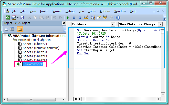
3. Poté tento kód uložte a zavřete a vraťte se do listu. Nyní, když vyberete buňku nebo výběr, budou vybrané buňky zvýrazněny a budou se dynamicky přesouvat při změně vybraných buněk.

Poznámky:

1. Pokud nemůžete najít Podokno Průzkumník projektu v okně můžete kliknout Pohled > Průzkumník projektu v Okno Microsoft Visual Basic pro aplikace otevřít.

2. Ve výše uvedeném kódu můžete změnit .ColorIndex = 6 barvu na jinou barvu, která se vám líbí.

3. Tento kód VBA lze použít na všechny listy v sešitu.

4. Pokud jsou v listu nějaké barevné buňky, barva se ztratí, když na buňku kliknete a poté přejdete do jiné buňky.


Související článek:

Jak automaticky zvýraznit řádek a sloupec aktivní buňky v aplikaci Excel?

Nejlepší nástroje pro produktivitu v kanceláři

🤖 Kutools AI asistent: Revoluční analýza dat založená na: Inteligentní provedení   |  Generovat kód  |  Vytvořte vlastní vzorce  |  Analyzujte data a generujte grafy  |  Vyvolejte funkce Kutools...
Populární funkce: Najít, zvýraznit nebo identifikovat duplikáty   |  Odstranit prázdné řádky   |  Kombinujte sloupce nebo buňky bez ztráty dat   |   Kolo bez vzorce ...
Super vyhledávání: Více kritérií VLookup    VLookup s více hodnotami  |   VLookup na více listech   |   Fuzzy vyhledávání ....
Pokročilý rozevírací seznam: Rychle vytvořte rozevírací seznam   |  Závislý rozbalovací seznam   |  Vícenásobný výběr rozevíracího seznamu ....
Správce sloupců: Přidejte konkrétní počet sloupců  |  Přesunout sloupce  |  Přepnout stav viditelnosti skrytých sloupců  |  Porovnejte rozsahy a sloupce ...
Doporučené funkce: Zaměření mřížky   |  Návrhové zobrazení   |   Velký Formula Bar    Správce sešitů a listů   |  Knihovna zdrojů (Automatický text)   |  Výběr data   |  Zkombinujte pracovní listy   |  Šifrovat/dešifrovat buňky    Odesílat e-maily podle seznamu   |  Super filtr   |   Speciální filtr (filtr tučné/kurzíva/přeškrtnuté...) ...
Top 15 sad nástrojů12 Text Tools (doplnit text, Odebrat znaky, ...)   |   50+ Graf Typ nemovitosti (Ganttův diagram, ...)   |   40+ Praktické Vzorce (Vypočítejte věk na základě narozenin, ...)   |   19 Vložení Tools (Vložte QR kód, Vložit obrázek z cesty, ...)   |   12 Konverze Tools (Čísla na slova, Přepočet měny, ...)   |   7 Sloučit a rozdělit Tools (Pokročilé kombinování řádků, Rozdělit buňky, ...)   |   ... a více

Rozšiřte své dovednosti Excel pomocí Kutools pro Excel a zažijte efektivitu jako nikdy předtím. Kutools for Excel nabízí více než 300 pokročilých funkcí pro zvýšení produktivity a úsporu času.  Kliknutím sem získáte funkci, kterou nejvíce potřebujete...

Popis


Office Tab přináší do Office rozhraní s kartami a usnadňuje vám práci

  • Povolte úpravy a čtení na kartách ve Wordu, Excelu, PowerPointu, Publisher, Access, Visio a Project.
  • Otevřete a vytvořte více dokumentů na nových kartách ve stejném okně, nikoli v nových oknech.
  • Zvyšuje vaši produktivitu o 50%a snižuje stovky kliknutí myší každý den!
Comments (16)
No ratings yet. Be the first to rate!
This comment was minimized by the moderator on the site
I had the same problem, read the whole page and comments. While thinking to apply it or not, I was just randomly clicking on number and letters to select the whole column and rows. Then suddenly highlight of selected cell feature came back :)
This comment was minimized by the moderator on the site
Hello, if someone can help me... I pick up this code in internet (apologies to the owner). It does almost what i need but this code select the entirerow. What i need is a change that alow to select just the first two cells of the row of the activecells. When i click in the cell, i need that the cell of the column "$I16" and "$J16" (16 is the first line of my table) of that row became interior color (=9359529). The code is this: 
Dim lTarget As Range

Private Sub Worksheet_SelectionChange(ByVal Target As Range)

If Target.Row >= 16 Then

If Not lTarget Is Nothing Then

lTarget.EntireRow.Interior.ColorIndex = 0
End If

Target.EntireRow.Interior.Color = 9359529

Set lTarget = Target
End If
End Sub

Can you help me? I had try to change this code but the only thing i can as the select the interior color of the cell target and not the column "$I" and "$J" in that specific row.Thank you for your help.
Luis Lopes
This comment was minimized by the moderator on the site
I know that you proposed a solution but the solution comes with another problem as you described below: "The only problem with having this code active is that you can no longer change the active cell color as it changes back to what it was before you clicked it. I suggest that if you need to change the highlight colors on the sheet, do so with macros disabled or change the sub name for a second so it doesn't trigger when you are clicking on cells". This is not an acceptable alternative for me. I need to be able to change the colors in the cells when the macro is active. Do you have a solution for this this problem. If you come up with a solution for this problem please republish your corrected macro the new macro in full (rather than proposing patches to your original macro because I am technically challenged as far as macro are concerned).
This comment was minimized by the moderator on the site
I tried your macro by copying and pasting it into my Excel file. I did change one thing in the macro though. I changed the color index from 6 to 24 (to a color different than the colors I am currently using in my macro). It worked very nicely and I liked it a lot but then started causing a problem for me. I have a lot of cells filled with with colors in my Excel. The macro started removing the color fill from every cell touched. I don't know how to stop the macro's this odd behavior. I did not have any choice but to remove the macro from my file. I still like to use this macro if someone can help me to fix it.
This comment was minimized by the moderator on the site
That was super helpful, thank you.
This comment was minimized by the moderator on the site
Anyway you can do the left adjacent cell to highlight instead of active cell? Or a range of cells around the activecell?
This comment was minimized by the moderator on the site
Thank you, but use this with caution. It has the undesirable counter effect of not letting undo. Is there any solution for that?
This comment was minimized by the moderator on the site
But i am unable to do undo option and lose the previously assigned cell color also.
Please provide solution
This comment was minimized by the moderator on the site
Perfect solution as I always tend to loose the track of the highlighted cell during "Find and Select" operation. Thanks a lot.
This comment was minimized by the moderator on the site
Great!! But what if I don't want to lose the previously assigned cell color? That would be greater to know.
This comment was minimized by the moderator on the site
Use a conditional format on the cells you want to protect.
This comment was minimized by the moderator on the site
Instead of "ColorIndex" which has a limited set of 255 values (meaning any custom colors are lost), use "Color" instead. You'll need to store the old value in a new static long variable and also generate the highlight color you want with the RGB function. The only problem with having this code active is that you can no longer change the active cell color as it changes back to what it was before you clicked it. I suggest that if you need to change the highlight colors on the sheet, do so with macros disabled or change the sub name for a second so it doesn't trigger when you are clicking on cells, then just rename it back to normal to "re-activate" it. Here is my code:

Sub Workbook_SheetSelectionChange(ByVal Sh As Object, ByVal Target As Excel.Range)

Static xLastRng As Range
Static xLastRngColor As Long

On Error Resume Next

xLastRng.Interior.Color = xLastRngColor
xLastRngColor = Target.Interior.Color
Target.Interior.Color = RGB(255, 255, 0) 'compose whatever highlight color you want with RGB values, I am using yellow here
Set xLastRng = Target

End Sub
This comment was minimized by the moderator on the site
work.... great...
This comment was minimized by the moderator on the site
Yes, I would like to know this as well. How would you keep the previously selected cells highlight for tracking purposes?
This comment was minimized by the moderator on the site
See my comment above.
There are no comments posted here yet
Load More
Please leave your comments in English
Posting as Guest
×
Rate this post:
0   Characters
Suggested Locations