Přejít k hlavnímu obsahu

Jak odkazovat na název karty v buňce v aplikaci Excel?

Chcete-li odkazovat na název aktuální záložky listu v buňce v aplikaci Excel, můžete to udělat pomocí vzorce nebo funkce Definovat uživatele. Tento výukový program vás provede následujícím způsobem.

Odkaz na aktuální název záložky listu v buňce pomocí vzorce
Odkaz na aktuální název záložky listu v buňce pomocí funkce Definovat uživatele
Pomocí Kutools pro Excel můžete snadno odkazovat na aktuální název záložky listu v buňce


Odkaz na aktuální název záložky listu v buňce pomocí vzorce

Při odkazování na název karty aktivního listu v konkrétní buňce v aplikaci Excel postupujte následovně.

1. Vyberte prázdnou buňku, zkopírujte a vložte vzorec = MID (CELL ("název souboru", A1), FIND ("]", CELL ("název souboru", A1)) + 1,255) do řádku vzorců a stiskněte vstoupit klíč. Viz snímek obrazovky:

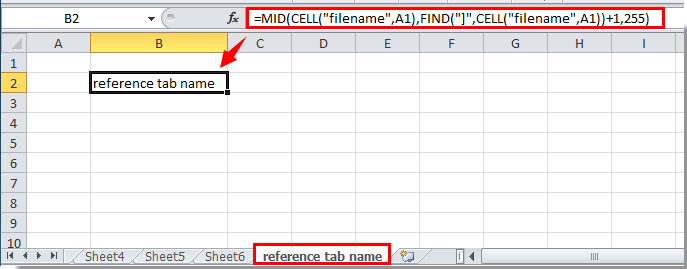
Nyní je v tabulce odkazován na název karty listu.

Snadno vložte název karty do konkrétní buňky, záhlaví nebo zápatí v listu:

Projekt Kutools pro Excel's Vložte informace o sešitu nástroj pomáhá snadno vložit název aktivní záložky do konkrétní buňky. Kromě toho můžete podle potřeby odkazovat na název sešitu, cestu sešitu, uživatelské jméno atd. Do buňky, záhlaví nebo zápatí listu. Klikněte pro detaily.
Stáhněte si Kutools pro Excel nyní! (30denní bezplatná trasa)


Odkaz na aktuální název záložky listu v buňce pomocí funkce Definovat uživatele

Kromě výše uvedené metody můžete odkazovat na název karty listu v buňce pomocí funkce Definovat uživatele.

1. lis Další + F11 k otevření Microsoft Visual Basic pro aplikace okno.

2. V Microsoft Visual Basic pro aplikace okno, klepněte na tlačítko Vložit > Modul. Viz snímek obrazovky:

3. Zkopírujte a vložte níže uvedený kód do okna Kód. A pak stiskněte Další + Q klávesy pro zavření Microsoft Visual Basic pro aplikace okno.

Kód VBA: název záložky odkazu

Function TabName()
  TabName = ActiveSheet.Name
End Function

4. Přejděte do buňky, kterou chcete odkazovat na název aktuální karty, zadejte = TabName () a potom stiskněte tlačítko vstoupit klíč. Poté se v buňce zobrazí aktuální název karty listu.


Odkazujte na aktuální název záložky listu v buňce pomocí Kutools pro Excel

S Vložte informace o sešitu užitečnost Kutools pro Excel, můžete snadno odkazovat na název karty listu v libovolné buňce, kterou chcete. Postupujte prosím následovně.

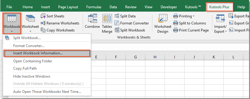
1. cvaknutí Kutools Plus > Cvičebnice > Vložte informace o sešitu. Viz snímek obrazovky:

2. V Vložte informace o sešitu dialogové okno vyberte Název listu v Informace sekci a v Vložte na vyberte sekci Rozsah a poté vyberte prázdnou buňku pro vyhledání názvu listu a nakonec klikněte na OK .

Můžete vidět, že název aktuálního listu je odkazován do vybrané buňky. Viz snímek obrazovky:

  Pokud chcete mít bezplatnou (30denní) zkušební verzi tohoto nástroje, kliknutím jej stáhněte, a poté přejděte k použití operace podle výše uvedených kroků.


Demo: Pomocí Kutools pro Excel můžete snadno odkazovat na aktuální název záložky listu v buňce

Kutools pro Excel obsahuje více než 300 užitečných nástrojů aplikace Excel. Zdarma to můžete vyzkoušet bez omezení do 30 dnů. Stáhněte si bezplatnou zkušební verzi hned teď!

Nejlepší nástroje pro produktivitu v kanceláři

🤖 Kutools AI asistent: Revoluční analýza dat založená na: Inteligentní provedení   |  Generovat kód  |  Vytvořte vlastní vzorce  |  Analyzujte data a generujte grafy  |  Vyvolejte funkce Kutools...
Populární funkce: Najít, zvýraznit nebo identifikovat duplikáty   |  Odstranit prázdné řádky   |  Kombinujte sloupce nebo buňky bez ztráty dat   |   Kolo bez vzorce ...
Super vyhledávání: Více kritérií VLookup    VLookup s více hodnotami  |   VLookup na více listech   |   Fuzzy vyhledávání ....
Pokročilý rozevírací seznam: Rychle vytvořte rozevírací seznam   |  Závislý rozbalovací seznam   |  Vícenásobný výběr rozevíracího seznamu ....
Správce sloupců: Přidejte konkrétní počet sloupců  |  Přesunout sloupce  |  Přepnout stav viditelnosti skrytých sloupců  |  Porovnejte rozsahy a sloupce ...
Doporučené funkce: Zaměření mřížky   |  Návrhové zobrazení   |   Velký Formula Bar    Správce sešitů a listů   |  Knihovna zdrojů (Automatický text)   |  Výběr data   |  Zkombinujte pracovní listy   |  Šifrovat/dešifrovat buňky    Odesílat e-maily podle seznamu   |  Super filtr   |   Speciální filtr (filtr tučné/kurzíva/přeškrtnuté...) ...
Top 15 sad nástrojů12 Text Tools (doplnit text, Odebrat znaky, ...)   |   50+ Graf Typ nemovitosti (Ganttův diagram, ...)   |   40+ Praktické Vzorce (Vypočítejte věk na základě narozenin, ...)   |   19 Vložení Tools (Vložte QR kód, Vložit obrázek z cesty, ...)   |   12 Konverze Tools (Čísla na slova, Přepočet měny, ...)   |   7 Sloučit a rozdělit Tools (Pokročilé kombinování řádků, Rozdělit buňky, ...)   |   ... a více

Rozšiřte své dovednosti Excel pomocí Kutools pro Excel a zažijte efektivitu jako nikdy předtím. Kutools for Excel nabízí více než 300 pokročilých funkcí pro zvýšení produktivity a úsporu času.  Kliknutím sem získáte funkci, kterou nejvíce potřebujete...

Popis


Office Tab přináší do Office rozhraní s kartami a usnadňuje vám práci

  • Povolte úpravy a čtení na kartách ve Wordu, Excelu, PowerPointu, Publisher, Access, Visio a Project.
  • Otevřete a vytvořte více dokumentů na nových kartách ve stejném okně, nikoli v nových oknech.
  • Zvyšuje vaši produktivitu o 50%a snižuje stovky kliknutí myší každý den!
Comments (24)
Rated 0.5 out of 5 · 1 ratings
This comment was minimized by the moderator on the site
sorry your formulas and everything are incorrect on this page.
after direct copy/paste your THEORIES were WRONG
ZERO OUT OF TWO ATTEMPTS WORKED USING YOUR SUGGESTIONS
Rated 0.5 out of 5
This comment was minimized by the moderator on the site
Hi Julia,
What kind of erro did you get?
To be mentioned, the formula provided in the post can only be applied in English system environment Excel. If you have Excel in a different language than English, please convert the formula from English to the language you are currently using.
You can translate the formula in this page: https://de.excel-translator.de/translator/
This comment was minimized by the moderator on the site
The formula at the top won't work until you save the file to your hard drive.
This comment was minimized by the moderator on the site
If you're using Excel Online. I found a solution for this issue.

You need to use 2 cells to make it work. As long as you have a cell that has the reference of a tab in its name, you can use FORMULATEXT() to turn that cells formula into a string and then extract the name that way. I can't imagine a scenario where you will want to reference another sheet and you wont already have a cell referencing that sheet for information on it, but you can always just make a blank/hidden (however you want to do it) cell that is just referencing the other sheet to set this formula up. In the below example, it is referencing cell B1 and cell B1 just contains =Sheet2!A1 as a reference to the sheet I want to name. If you use a name for a sheet with a space in it (example: Sheet 1) it would show up as (='Sheet 1'A1). I used an IF function and an ISERROR function to search if the string contains a space or not and two MID functions to extract the name of the sheet from both scenarios. If you update the name of the referenced sheet, cell B1 will change its formula and subsequently change the string and output the correct name each time.

=IF(ISERROR(FIND(" ",FORMULATEXT(B1))),MID(FORMULATEXT(B1),2,FIND("!",FORMULATEXT(B1))-2),MID(FORMULATEXT(B1),3,FIND("!",FORMULATEXT(B1))-4))
This comment was minimized by the moderator on the site
What I really want is to name some tabs using with the names on some cells from another sheet (same document of course). How can I do that?
This comment was minimized by the moderator on the site
Hi, I used the above suggestions but the first formula to reference the tab sheet name will not work on "excel" online. The second works, but the "Tabname" keeps showing the same tab name for all tabs on the workbook.
This comment was minimized by the moderator on the site
Hi,
Sorry we didn't test in excel online. Can't help you with that yet. Thank you for your comment.
This comment was minimized by the moderator on the site
hello, i am having trouble referencing a sheet name into a cell with online excel
This comment was minimized by the moderator on the site
Excellent, thanks! Per: Reference the current sheet tab name in cell with formula
This comment was minimized by the moderator on the site
Sorry, the comment line is wrong - should be Ctrl-Alt-Shift-F9
This comment was minimized by the moderator on the site
FYI, you need to have more than one sheet in your workbook for this to work. Otherwise, the formula will display the filename but no sheet name.
This comment was minimized by the moderator on the site
Good Day,
Thank you for your comment. I have tested the formula in a workbook that has only one sheet, but everything was running smoothly. The formula only displays the sheet name no matter how many worksheets existing in a workbook.
There are no comments posted here yet
Load More
Please leave your comments in English
Posting as Guest
×
Rate this post:
0   Characters
Suggested Locations