Jak skrýt pouze část hodnoty buňky v aplikaci Excel?

Předpokládejme, že máte list s některými obecnými informacemi o personálu, ale některé jsou soukromé, například čísla sociálního zabezpečení. Nyní chcete skrýt část těchto čísel sociálního zabezpečení, jak je uvedeno níže, jak to můžete rychle vyřešit?

Částečně skryjte čísla sociálního zabezpečení pomocí Format Cells

Částečně skryjte text nebo číslo pomocí vzorců

Částečně skryjte čísla sociálního zabezpečení pomocí Format Cells

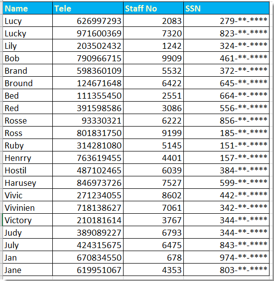
Chcete-li skrýt část čísel sociálního zabezpečení v aplikaci Excel, můžete to vyřešit pomocí Formát buněk.

1. Vyberte čísla, která chcete částečně skrýt, a vyberte je kliknutím pravým tlačítkem Formát buněk z kontextového menu. Viz screenshot:

2. Pak v Formát buněk dialog, klepněte na tlačítko Číslo Záložka a zvolte Zvyk od Kategorie v podokně a přejděte do této položky 000 ,, "- ** - ****" do Styl pole v pravé části. Viz snímek obrazovky:

3. cvaknutí OK, nyní byla skryta dílčí čísla, která jste vybrali.

Poznámka： Zaokrouhlí číslo nahoru, pokud je čtvrté číslo větší než nebo eaqul na 5.

Částečně skryjte text nebo číslo pomocí vzorců

U výše uvedené metody můžete skrýt pouze částečná čísla, pokud chcete skrýt částečná čísla nebo texty, postupujte takto:

Zde skryjeme první 4 čísla čísla pasu.

Vyberte jednu prázdnou buňku vedle čísla pasu, například F22, zadejte tento vzorec = "****" & VPRAVO (E22,5)a potom přetáhněte úchyt automatického vyplňování přes buňku, kterou potřebujete k použití tohoto vzorce.

Tip:

Pokud chcete skrýt poslední čtyři čísla, použijte tento vzorec, = VLEVO (H2,5) & "****"

Pokud chcete skrýt prostřední tři čísla, použijte toto = VLEVO (H2,3) & "***" & VPRAVO (H2,3)

Nejlepší nástroje pro produktivitu v kanceláři

🤖	Kutools AI asistent: Revoluční analýza dat založená na: Inteligentní provedení   |  Generovat kód  |  Vytvořte vlastní vzorce  |  Analyzujte data a generujte grafy  |  Vyvolejte funkce Kutools...
	Populární funkce: Najít, zvýraznit nebo identifikovat duplikáty   |  Odstranit prázdné řádky   |  Kombinujte sloupce nebo buňky bez ztráty dat   |   Kolo bez vzorce ...
	Super vyhledávání: Více kritérií VLookup  |   VLookup s více hodnotami  |   VLookup na více listech   |   Fuzzy vyhledávání ....
	Pokročilý rozevírací seznam: Rychle vytvořte rozevírací seznam   |  Závislý rozbalovací seznam   |  Vícenásobný výběr rozevíracího seznamu ....
	Správce sloupců: Přidejte konkrétní počet sloupců  |  Přesunout sloupce  |  Přepnout stav viditelnosti skrytých sloupců  |  Porovnejte rozsahy a sloupce ...
	Doporučené funkce: Zaměření mřížky   |  Návrhové zobrazení   |   Velký Formula Bar   |  Správce sešitů a listů   |  Knihovna zdrojů (Automatický text)   |  Výběr data   |  Zkombinujte pracovní listy   |  Šifrovat/dešifrovat buňky   |  Odesílat e-maily podle seznamu   |  Super filtr   |   Speciální filtr (filtr tučné/kurzíva/přeškrtnuté...) ...
	Top 15 sad nástrojů:  12 Text Tools (doplnit text, Odebrat znaky, ...)   |   50+ Graf Typ nemovitosti (Ganttův diagram, ...)   |   40+ Praktické Vzorce (Vypočítejte věk na základě narozenin, ...)   |   19 Vložení Tools (Vložte QR kód, Vložit obrázek z cesty, ...)   |   12 Konverze Tools (Čísla na slova, Přepočet měny, ...)   |   7 Sloučit a rozdělit Tools (Pokročilé kombinování řádků, Rozdělit buňky, ...)   |   ... a více

Rozšiřte své dovednosti Excel pomocí Kutools pro Excel a zažijte efektivitu jako nikdy předtím. Kutools for Excel nabízí více než 300 pokročilých funkcí pro zvýšení produktivity a úsporu času.  Kliknutím sem získáte funkci, kterou nejvíce potřebujete...

Čtěte více... Stažení zdarma...

---

Office Tab přináší do Office rozhraní s kartami a usnadňuje vám práci

• Povolte úpravy a čtení na kartách ve Wordu, Excelu, PowerPointu, Publisher, Access, Visio a Project.
• Otevřete a vytvořte více dokumentů na nových kartách ve stejném okně, nikoli v nových oknech.
• Zvyšuje vaši produktivitu o 50%a snižuje stovky kliknutí myší každý den!

Čtěte více... Stažení zdarma...