Přejít k hlavnímu obsahu

Jak vytvořit rozevírací seznam s více zaškrtávacími políčky v aplikaci Excel?

Mnoho uživatelů aplikace Excel má tendenci vytvářet rozevírací seznam s více zaškrtávacími políčky, aby vybrali více položek ze seznamu najednou. Ve skutečnosti nemůžete vytvořit seznam s více zaškrtávacími políčky pomocí Ověření dat. V tomto kurzu vám ukážeme dvě metody vytvoření rozevíracího seznamu s více zaškrtávacími políčky v aplikaci Excel.

Pomocí seznamu vytvořte rozevírací seznam s více zaškrtávacími políčky
Odpověď: Vytvořte seznam se zdrojovými daty
B: Pojmenujte buňku, ve které najdete vybrané položky
C: Vložte tvar, který pomůže výstupu vybraných položek
Snadno vytvářejte rozevírací seznam se zaškrtávacími políčky pomocí úžasného nástroje
Další výukové programy pro rozevírací seznam ...


Pomocí seznamu vytvořte rozevírací seznam s více zaškrtávacími políčky

Jak je ukázáno níže, v aktuálním listu budou zdrojovými daty seznamu všechny názvy v rozsahu A2: A11. Kliknutím na tlačítko v buňce C4 můžete vypsat vybrané položky a všechny vybrané položky v seznamu se zobrazí v buňce E4. K dosažení tohoto cíle postupujte následovně.

A. Vytvořte seznam se zdrojovými daty

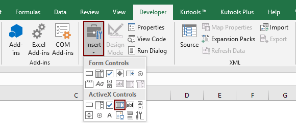
1. cvaknutí Vývojka > Vložit > Seznam (ovládací prvek Active X). Viz snímek obrazovky:

2. Nakreslete seznam do aktuálního listu, klikněte na něj pravým tlačítkem a vyberte Nemovitosti z nabídky pravého tlačítka myši.

3. V Nemovitosti dialogové okno, musíte nakonfigurovat následujícím způsobem.

  • 3.1 V ListFillRange do pole zadejte rozsah zdroje, který se zobrazí v seznamu (zde zadám rozsah A2: A11);
  • 3.2 V ListStyle zaškrtněte políčko 1 - Volba stylu fmList;
  • 3.3 V Více násobný výběr zaškrtněte políčko 1 - fmMultiSelectMulti;
  • 3.4 Zavřete Nemovitosti dialogové okno. Viz snímek obrazovky:

B: Pojmenujte buňku, ve které najdete vybrané položky

Pokud potřebujete odeslat všechny vybrané položky do určené buňky, například E4, postupujte následovně.

1. Vyberte buňku E4, zadejte ListBoxOutput do Název Box a stiskněte tlačítko vstoupit klíč.

C. Vložte tvar, který pomůže výstupu vybraných položek

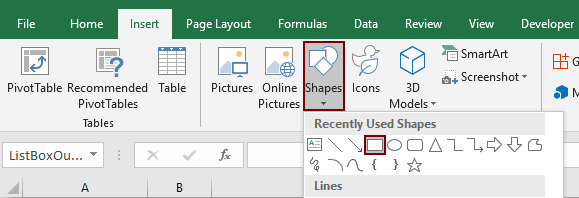
1. cvaknutí Vložit > Tvary > Obdélník. Viz obrázek:

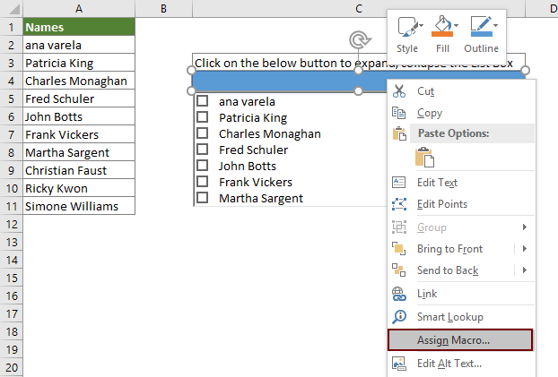
2. Nakreslete do listu obdélník (zde nakreslím obdélník do buňky C4). Poté klikněte pravým tlačítkem na obdélník a vyberte Přiřadit makro z nabídky pravého tlačítka myši.

3. V Přiřadit makro dialogové okno, klepněte na tlačítko Nový .

4. V otvoru Microsoft Visual Basic pro aplikace v okně, nahraďte prosím původní kód v Modul okno s níže uvedeným kódem VBA.

Kód VBA: Vytvořte seznam s více zaškrtávacími políčky

Sub Rectangle1_Click()
'Updated by Extendoffice 20200730
Dim xSelShp As Shape, xSelLst As Variant, I, J As Integer
Dim xV As String
Set xSelShp = ActiveSheet.Shapes(Application.Caller)
Set xLstBox = ActiveSheet.ListBox1
If xLstBox.Visible = False Then
    xLstBox.Visible = True
    xSelShp.TextFrame2.TextRange.Characters.Text = "Pickup Options"
    xStr = ""
    xStr = Range("ListBoxOutput").Value
    
    If xStr <> "" Then
         xArr = Split(xStr, ";")
    For I = xLstBox.ListCount - 1 To 0 Step -1
        xV = xLstBox.List(I)
        For J = 0 To UBound(xArr)
            If xArr(J) = xV Then
              xLstBox.Selected(I) = True
              Exit For
            End If
        Next
    Next I
    End If
Else
    xLstBox.Visible = False
    xSelShp.TextFrame2.TextRange.Characters.Text = "Select Options"
    For I = xLstBox.ListCount - 1 To 0 Step -1
        If xLstBox.Selected(I) = True Then
        xSelLst = xLstBox.List(I) & ";" & xSelLst
        End If
    Next I
    If xSelLst <> "" Then
        Range("ListBoxOutput") = Mid(xSelLst, 1, Len(xSelLst) - 1)
    Else
        Range("ListBoxOutput") = ""
    End If
End If
End Sub

Poznámka: V kódu Obdélník 1 je název tvaru; ListBox1 je název seznamu; Zvolte Volby a Možnosti vyzvednutí jsou zobrazené texty tvaru; a ListBoxOutput je název rozsahu výstupní buňky. Můžete je změnit podle svých potřeb.

5. lis Další + Q současně zavřete Microsoft Visual Basic pro aplikace okno.

6. Kliknutím na tlačítko obdélníku rozbalíte nebo rozbalíte seznam. Když se seznam rozšiřuje, zkontrolujte položky v seznamu a poté znovu klikněte na obdélník, aby se všechny vybrané položky zobrazily do buňky E4. Viz níže demo:

7. A potom uložte sešit jako Sešit Excel MacroEnable pro opětovné použití kódu v budoucnu.


Vytvořte rozevírací seznam se zaškrtávacími políčky s úžasným nástrojem

Výše uvedená metoda je příliš vícestupňová, než aby ji bylo možné snadno zpracovat. Zde velmi doporučujeme Rozevírací seznam se zaškrtávacími políčky užitečnost Kutools pro vynikat které vám pomohou snadno vytvořit rozevírací seznam se zaškrtávacími políčky v zadaném rozsahu, aktuálním listu, aktuálním sešitu nebo všech otevřených sešitech podle vašich potřeb. Podívejte se na níže uvedenou ukázku:
Stáhněte si a vyzkoušejte! (30denní bezplatná trasa)

Kromě výše uvedeného dema poskytujeme také podrobného průvodce, který ukazuje, jak použít tuto funkci k dosažení tohoto úkolu. Postupujte prosím následovně.

1. Otevřete list, který jste nastavili v rozevíracím seznamu pro ověření dat, klikněte na Kutools > Rozbalovací seznam > Rozevírací seznam se zaškrtávacími políčky > Nastavení. Viz obrázek:

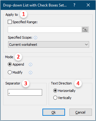
2. V Rozevírací seznam s nastavením zaškrtávacích políček V dialogovém okně proveďte následující konfiguraci.

  • 2.1) V Naneste na V části zadejte rozsah použití, kde vytvoříte zaškrtávací políčka pro položky v rozevíracím seznamu. Můžete zadat a určitý rozsah, aktuální list, aktuální sešit or všechny otevřené sešity na základě vašich potřeb.
  • 2.2) V režim sekce, vyberte styl, kterým chcete vypsat vybrané položky;
  • Tady je Upravit jako příklad, pokud zvolíte toto, hodnota buňky se změní na základě vybraných položek.
  • 2.3) V oddělovač do pole zadejte oddělovač, který použijete k oddělení více položek;
  • 2.4) V Směr textu sekce vyberte směr textu podle svých potřeb;
  • 2.5) Klikněte na OK .

3. V posledním kroku klikněte na Kutools > Rozbalovací seznam > Rozevírací seznam se zaškrtávacími políčky > Povolit rozevírací seznam zaškrtávacích políček aktivovat tuto funkci.

Od nynějška, když kliknete na buňky s rozevíracím seznamem ve specifikovaném rozsahu, zobrazí se seznamové pole. Vyberte položky zaškrtnutím políček pro výstup do buňky, jak je ukázáno níže (ukázka je režim úprav) ).

Další podrobnosti o této funkci prosím navštivte zde.

  Pokud chcete mít bezplatnou (30denní) zkušební verzi tohoto nástroje, kliknutím jej stáhněte, a poté přejděte k použití operace podle výše uvedených kroků.


Související články:

Automatické doplňování při psaní v rozevíracím seznamu aplikace Excel
Pokud máte rozevírací seznam pro ověření dat s velkými hodnotami, musíte v seznamu posunout dolů, abyste našli ten správný, nebo přímo zadat celé slovo do seznamu. Pokud existuje metoda umožňující automatické dokončení při psaní prvního písmene do rozevíracího seznamu, vše bude jednodušší. Tento výukový program poskytuje způsob řešení problému.

Vytvořte rozevírací seznam z jiného sešitu v aplikaci Excel
Je docela snadné vytvořit rozevírací seznam pro ověření dat mezi listy v sešitu. Ale pokud se seznamová data, která potřebujete pro ověření dat, nacházejí v jiném sešitu, co byste udělali? V tomto kurzu se naučíte, jak vytvořit seznam drop fown z jiného sešitu v aplikaci Excel podrobně.

Vytvořte prohledávatelný rozevírací seznam v aplikaci Excel
Pro rozevírací seznam s mnoha hodnotami není hledání správné práce snadná práce. Dříve jsme zavedli způsob automatického vyplňování rozevíracího seznamu při zadávání prvního písmene do rozevíracího seznamu. Kromě funkce automatického doplňování můžete také v rozevíracím seznamu vyhledávat, abyste zvýšili efektivitu práce při hledání správných hodnot v rozevíracím seznamu. Chcete-li v rozevíracím seznamu vyhledávat, vyzkoušejte metodu v tomto kurzu.

Automatické vyplnění dalších buněk při výběru hodnot v rozevíracím seznamu aplikace Excel
Řekněme, že jste vytvořili rozevírací seznam na základě hodnot v oblasti buněk B8: B14. Když vyberete libovolnou hodnotu z rozevíracího seznamu, chcete, aby se ve vybrané buňce automaticky naplnily odpovídající hodnoty v rozsahu buněk C8: C14. Při řešení problému vám metody v tomto tutoriálu udělají laskavost.

Další výukové programy pro rozevírací seznam ...

Nejlepší nástroje pro produktivitu v kanceláři

🤖 Kutools AI asistent: Revoluční analýza dat založená na: Inteligentní provedení   |  Generovat kód  |  Vytvořte vlastní vzorce  |  Analyzujte data a generujte grafy  |  Vyvolejte funkce Kutools...
Populární funkce: Najít, zvýraznit nebo identifikovat duplikáty   |  Odstranit prázdné řádky   |  Kombinujte sloupce nebo buňky bez ztráty dat   |   Kolo bez vzorce ...
Super vyhledávání: Více kritérií VLookup    VLookup s více hodnotami  |   VLookup na více listech   |   Fuzzy vyhledávání ....
Pokročilý rozevírací seznam: Rychle vytvořte rozevírací seznam   |  Závislý rozbalovací seznam   |  Vícenásobný výběr rozevíracího seznamu ....
Správce sloupců: Přidejte konkrétní počet sloupců  |  Přesunout sloupce  |  Přepnout stav viditelnosti skrytých sloupců  |  Porovnejte rozsahy a sloupce ...
Doporučené funkce: Zaměření mřížky   |  Návrhové zobrazení   |   Velký Formula Bar    Správce sešitů a listů   |  Knihovna zdrojů (Automatický text)   |  Výběr data   |  Zkombinujte pracovní listy   |  Šifrovat/dešifrovat buňky    Odesílat e-maily podle seznamu   |  Super filtr   |   Speciální filtr (filtr tučné/kurzíva/přeškrtnuté...) ...
Top 15 sad nástrojů12 Text Tools (doplnit text, Odebrat znaky, ...)   |   50+ Graf Typ nemovitosti (Ganttův diagram, ...)   |   40+ Praktické Vzorce (Vypočítejte věk na základě narozenin, ...)   |   19 Vložení Tools (Vložte QR kód, Vložit obrázek z cesty, ...)   |   12 Konverze Tools (Čísla na slova, Přepočet měny, ...)   |   7 Sloučit a rozdělit Tools (Pokročilé kombinování řádků, Rozdělit buňky, ...)   |   ... a více

Rozšiřte své dovednosti Excel pomocí Kutools pro Excel a zažijte efektivitu jako nikdy předtím. Kutools for Excel nabízí více než 300 pokročilých funkcí pro zvýšení produktivity a úsporu času.  Kliknutím sem získáte funkci, kterou nejvíce potřebujete...

Popis


Office Tab přináší do Office rozhraní s kartami a usnadňuje vám práci

  • Povolte úpravy a čtení na kartách ve Wordu, Excelu, PowerPointu, Publisher, Access, Visio a Project.
  • Otevřete a vytvořte více dokumentů na nových kartách ve stejném okně, nikoli v nových oknech.
  • Zvyšuje vaši produktivitu o 50%a snižuje stovky kliknutí myší každý den!
Comments (70)
No ratings yet. Be the first to rate!
This comment was minimized by the moderator on the site
Hello-

This is fabulous, but I was wondering if there is a way to call the code as a subroutine, ie Click Button 1, run this code with X List Box and X Output cell. I want to pass the listbox and the output cell as variables into this code. Any help would be greatly appreciated.

I've tried this:
Private Sub Rectangle1_Click()
Call MultiSelctDropdown(ListBox1,Output1)
End Sub

Private Sub Rectangle2_Click()
Call MultiSelctDropdown(ListBox2,Output2)
End Sub

Private Sub MultiSelectDropdown(ListBox As String, Output As String)
Dim xSelShp As Shape, xSelLst As Variant, I, J As Integer
Dim xV As String
Set xSelShp = ActiveSheet.Shapes(Application.Caller)
Set xLstBox = ActiveSheet.ListBox
If xLstBox.Visible = False Then
xLstBox.Visible = True
xSelShp.TextFrame2.TextRange.Characters.Text = "Enter"
xStr = ""
xStr = Range("Output").Value

If xStr <> "" Then
xArr = Split(xStr, ",")
For I = xLstBox.ListCount - 1 To 0 Step -1
xV = xLstBox.List(I)
For J = 0 To UBound(xArr)
If xArr(J) = xV Then
xLstBox.Selected(I) = True
Exit For
End If
Next
Next I
End If
Else
xLstBox.Visible = False
xSelShp.TextFrame2.TextRange.Characters.Text = "Click Here to Select Products"
For I = xLstBox.ListCount - 1 To 0 Step -1
If xLstBox.Selected(I) = True Then
xSelLst = xLstBox.List(I) & "," & xSelLst
End If
Next I
If xSelLst <> "" Then
Range("Output") = Mid(xSelLst, 1, Len(xSelLst) - 1)
Else
Range("Output") = ""
End If
End If
End Sub
This comment was minimized by the moderator on the site
Ok I figured this one out (see below)

But now I want to have only ONE list box that I can use over and over again with different buttons but different output depending on the button pushed. And the code below works for this EXCEPT the items selected when the list box pops up includes all items that have been outputted from the code.

If list box1 contains

Apples
Oranges
Pears
Kiwi

and button 1 is pressed and Apples is selected, when button 2 is pressed Apples is already selected, and if during button press 2 pears is selected when you go back to button 1 Apples AND Pears are selected.

How can I either clear all selected when a button is pressed OR make the selected options equal to the output.


Private Sub Button1_Click()
Call ProductSelection(ActiveSheet.ListBox1, "Button1Output", 243, 215)
End Sub
Private Sub Button2_Click()
Call ProductSelection(ActiveSheet.ListBox1, "Button2Output", 472, 215)
End Sub


Private Sub ProductSelection(xListBox As Object, Output As String, left As Integer, height As Integer)
Dim xSelShp As Shape, xSelLst As Variant, I, J As Integer
Dim xV As String
Set xSelShp = ActiveSheet.Shapes(Application.Caller)
Set xLstBox = xListBox
If xLstBox.Visible = False Then
xLstBox.Visible = True
xLstBox.left = left
xLstBox.height = height
xSelShp.TextFrame2.TextRange.Characters.Text = "Enter"
xStr = ""
xStr = Range(Output).Value

If xStr <> "" Then
xArr = Split(xStr, ",")
For I = xLstBox.ListCount - 1 To 0 Step -1
xV = xLstBox.List(I)
For J = 0 To UBound(xArr)
If xArr(J) = xV Then
xLstBox.Selected(I) = True
Exit For
End If
Next
Next I
End If
Else
xLstBox.Visible = False
xSelShp.TextFrame2.TextRange.Characters.Text = "Click Here to Select Products"
For I = xLstBox.ListCount - 1 To 0 Step -1
If xLstBox.Selected(I) = True Then
xSelLst = xLstBox.List(I) & "," & xSelLst
End If
Next I
If xSelLst <> "" Then
Range(Output) = Mid(xSelLst, 1, Len(xSelLst) - 1)
Else
Range(Output) = ""
End If
End If
End Sub
This comment was minimized by the moderator on the site
Hi there- this is super helpful, thank you! Can you tell me how I can draw a list box based on a list in a different worksheet (but same file)? I've tried entering my worksheet name (i.e., 'lists') followed by the range in the list fill range (after clicking on Properties) but this does not work.Thanks!
This comment was minimized by the moderator on the site
Hi Meghan,Supposing you want to <span style="letter-spacing: 0.2px; color: inherit; font-family: inherit; font-style: inherit; font-variant-ligatures: inherit; font-variant-caps: inherit;">ListBox1</span><span style="letter-spacing: 0.2px; color: inherit; font-family: inherit; font-style: inherit; font-variant-ligatures: inherit; font-variant-caps: inherit;">Sheet1</span><div data-tag="code">Sub listboxlistfillrangefromdifferentsheet()
Sheet1.ListBox1.ListFillRange = Sheet2.Range("A2:A20").Address(, , , True)
End Sub
This comment was minimized by the moderator on the site
hello, I have a problem with the list box: to make the list going down, I have to click on the box that allows the list to go down but when I click, it does not go down automatically, I have to click outside the list so that it refreshes and the list goes down, what to do? Thank you
This comment was minimized by the moderator on the site
Hi,You can't scroll ActiveX Listbox by mouse wheel. There is no setting for it.

This comment was minimized by the moderator on the site
Hi, thank you for sharing this! I have a question though, is it possible to populate different cells based on the selected option?For example, instead of having everything in one cell, each selection is populated in the cell below the earlier selection. Thank you!
This comment was minimized by the moderator on the site
Hi faez,
The VBA below helps to populate the selected options in different cells on the same row. Please have a try.

Sub Rectangle2_Click()
'Updated by Extendoffice 20211124
Dim xSelShp As Shape, xSelLst As Variant, I As Integer
Dim xRg As Range
Set xSelShp = ActiveSheet.Shapes(Application.Caller)
Set xLstBox = ActiveSheet.ListBox1
If xLstBox.Visible = False Then
xLstBox.Visible = True
xSelShp.TextFrame2.TextRange.Characters.Text = "Pickup Options"
Else
xLstBox.Visible = False
xSelShp.TextFrame2.TextRange.Characters.Text = "Select Options"
Set xRg = Range("ListBoxOutput")
For I = 0 To xLstBox.ListCount - 1
If xLstBox.Selected(I) = True Then
xSelLst = xLstBox.List(I)
xRg.Value = Mid(xSelLst, 1, Len(xSelLst))
Set xRg = xRg.Offset(0, 1)
End If
Next I
End If
End Sub
This comment was minimized by the moderator on the site
Hi Crystal,
Thanks a lot for this code, very helpful and convenient. One question : how to adpat it in order not to have the separator ";" if only one item is selected ?
This comment was minimized by the moderator on the site
Hi Eloi,No separator is displayed when you select only one item in the list.
This comment was minimized by the moderator on the site
Thanks Crystal, the mistake was in my adaptation of the code.
If someone needs to adapt it with a click on a cell instead of a click on a shape, you could try this (with a call to this sub in your sheet, with a condition when your cell is selected)

Sub affichage_liste(xLstBox As MSForms.ListBox, texte1 As String)
'Updated by Extendoffice 20200730
Dim xSelLst As Variant, I, J As Integer
Dim xV As String

If xLstBox.Visible = False Then
xLstBox.Visible = True
xStr = ""
xStr = Range(texte1).Value

If xStr <> "" Then
xArr = Split(xStr, ";")
For I = xLstBox.ListCount - 1 To 0 Step -1
xV = xLstBox.List(I)
For J = 0 To UBound(xArr)
If xArr(J) = xV Then
xLstBox.Selected(I) = True
Exit For
End If
Next
Next I
End If
Else
xLstBox.Visible = False
For I = xLstBox.ListCount - 1 To 0 Step -1
If xLstBox.Selected(I) = True Then
xSelLst = xLstBox.List(I) & "; " & xSelLst
End If
Next I
If xSelLst <> "" Then
Range(texte1) = Mid(xSelLst, 1, Len(xSelLst) - 2)
Else
Range(texte1) = ""
End If
End If
End Sub
This comment was minimized by the moderator on the site
Hi Eloi,The code you provided doesn't seem to work. I have modified it again as below.  After adding the code in your Sheet(Code) window, go back to the worksheet, click the cell C4 to expand the list box, after selecting items from the list box, click on any cell in the worksheet to output the selection, and no separator is displayed when you select only one item in the list.
<div data-tag="code">Private Sub Worksheet_SelectionChange(ByVal Target As Range)
'Updated by Extendoffice 20211223
Dim xSelLst As Variant, I, J As Integer
Dim xV As String
Set xLstBox = ActiveSheet.ListBox1

If Target.Address = "$C$4" Then


If xLstBox.Visible = False Then
xLstBox.Visible = True
xStr = ""
xStr = Range("ListBoxOutput").Value

If xStr <> "" Then
xArr = Split(xStr, ";")
For I = xLstBox.ListCount - 1 To 0 Step -1
xV = xLstBox.List(I)
For J = 0 To UBound(xArr)
If xArr(J) = xV Then
xLstBox.Selected(I) = True
Exit For
End If
Next
Next I
End If

End If

Else
xLstBox.Visible = False

For I = xLstBox.ListCount - 1 To 0 Step -1
If xLstBox.Selected(I) = True Then
xSelLst = xLstBox.List(I) & "; " & xSelLst
End If
Next I
If xSelLst <> "" Then
Range("ListBoxOutput") = Mid(xSelLst, 1, Len(xSelLst) - 2)
Else
Range("ListBoxOutput") = ""
End If


End If

End Sub
This comment was minimized by the moderator on the site
Thanks a lot Crystal
This comment was minimized by the moderator on the site
Bonjour,Je suis plus que novice sur excel étant sur mac je ne peux utiliser l'outil Kutools j'ai donc tenté de créer une liste déroulante où l'on peut cocher plusieurs items mais je bloque dès le début dans l'onglet développeur puisque je n'ai pas du tout l'outil "insert".Merci pour votre aide
This comment was minimized by the moderator on the site
Hi I am newbie to VBA. I tried to execute the code but i get the following error "Run-time error '-2147024809 (80070057)': The Item with the specified name wasn't found". Can you help me with this
This comment was minimized by the moderator on the site
Hi Gowtham,It seem that this error occurs when you running the code directly in the Code editor (the Microsoft Visual Basic for Applications window).After adding the code, please press the Alt + Q keys to close the Microsoft Visual Basic for Applications window. Go back to the worksheet and execute the code by clicking the rectangle button (see the .gif picture in step 6).
This comment was minimized by the moderator on the site
Hi Crystal, even after your tip am getting same error as Gowtham. My error is right after protect my sheet. Would you please help me with this issue?
This comment was minimized by the moderator on the site
Hi Crystal, Even After your tip I am getting same error as Gowtham.
This comment was minimized by the moderator on the site
Hi Mina,Which Excel and Windows version are you using?
This comment was minimized by the moderator on the site
Hello,I added this code to an existing macro template and it is loading the selections correctly, but it is NOT clearing out the x on the selected items..This will be used on/in a template worksheet that has submit button/macro to load the worksheet answers into a hidden worksheet with a data table.And am happy to say the field data loaded to the cell, transferred into my variable, and loaded to the data table as expected.
This code was a HUGE blessing!
I use excel 2016
How do I fix this. I am using this version from below.
Sub Rectangle1_Click()
'Updated by Extendoffice 20200730
Dim xSelShp As Shape, xSelLst As Variant, I, J As Integer
Dim xV As String
Set xSelShp = ActiveSheet.Shapes(Application.Caller)
Set xLstBox = ActiveSheet.ListBox1
If xLstBox.Visible = False Then
xLstBox.Visible = True
xSelShp.TextFrame2.TextRange.Characters.Text = "Pickup Options"
xStr = ""
xStr = Range("ListBoxOutput").Value

If xStr <> "" Then
xArr = Split(xStr, ";")
For I = xLstBox.ListCount - 1 To 0 Step -1
xV = xLstBox.List(I)
For J = 0 To UBound(xArr)
If xArr(J) = xV Then
xLstBox.Selected(I) = True
Exit For
End If
Next
Next I
End If
Else
xLstBox.Visible = False
xSelShp.TextFrame2.TextRange.Characters.Text = "Select Options"
For I = xLstBox.ListCount - 1 To 0 Step -1
If xLstBox.Selected(I) = True Then
xSelLst = xLstBox.List(I) & ";" & xSelLst
End If
Next I
If xSelLst <> "" Then
Range("ListBoxOutput") = Mid(xSelLst, 1, Len(xSelLst) - 1)
Else
Range("ListBoxOutput") = ""
End If
End If
End Sub
This comment was minimized by the moderator on the site
Hello,

I'm having a similar problem to Tom from 2 months ago. When I try to share my file with a colleague, the multi-select droplist list isn't working. However, I used the Kutools add-on to create this as opposed to creating it myself. I've also saved it as macro-enabled.
This comment was minimized by the moderator on the site
Hi ben,The multi-select drop down list feature of Kutools only works in the Excel that installed our Kutools. We are working on this issue, sorry for the inconvenience.
This comment was minimized by the moderator on the site
Hello I looking the resolve for problem with saving choosing on drop down list

when i choose something on list and send file to my colleague, then when he open file and want to check my list then list has cleared and cell "ListBoxOutput" was cleared too.

help please :)
This comment was minimized by the moderator on the site
Hi Tom,
Please save the workbook as an "Excel MacroEnable Workbook" and then send this .xlsm file to your colleague.
This comment was minimized by the moderator on the site
hello i save this file in this format from beginning ;), but without effect. still when i fill file and send to someone then when he opened file and click to "shape" then macro started from begin and cleared list
This comment was minimized by the moderator on the site
Hi Tom,
I am sorry for the mistake. The code has been updated again. Please have a try.

Sub Rectangle1_Click()

'Updated by Extendoffice 20200730

Dim xSelShp As Shape, xSelLst As Variant, I, J As Integer

Dim xV As String

Set xSelShp = ActiveSheet.Shapes(Application.Caller)

Set xLstBox = ActiveSheet.ListBox1

If xLstBox.Visible = False Then

xLstBox.Visible = True

xSelShp.TextFrame2.TextRange.Characters.Text = "Pickup Options"

xStr = ""

xStr = Range("ListBoxOutput").Value


If xStr <> "" Then

xArr = Split(xStr, ";")

For I = xLstBox.ListCount - 1 To 0 Step -1

xV = xLstBox.List(I)

For J = 0 To UBound(xArr)

If xArr(J) = xV Then

xLstBox.Selected(I) = True

Exit For

End If

Next

Next I

End If

Else

xLstBox.Visible = False

xSelShp.TextFrame2.TextRange.Characters.Text = "Select Options"

For I = xLstBox.ListCount - 1 To 0 Step -1

If xLstBox.Selected(I) = True Then

xSelLst = xLstBox.List(I) & ";" & xSelLst

End If

Next I

If xSelLst <> "" Then

Range("ListBoxOutput") = Mid(xSelLst, 1, Len(xSelLst) - 1)

Else

Range("ListBoxOutput") = ""

End If

End If

End Sub
This comment was minimized by the moderator on the site
Now it's working perfectly.

Many thanks for your help
There are no comments posted here yet
Load More
Please leave your comments in English
Posting as Guest
×
Rate this post:
0   Characters
Suggested Locations