Přejít k hlavnímu obsahu

Jak sčítat na základě kritérií sloupců a řádků v aplikaci Excel? 

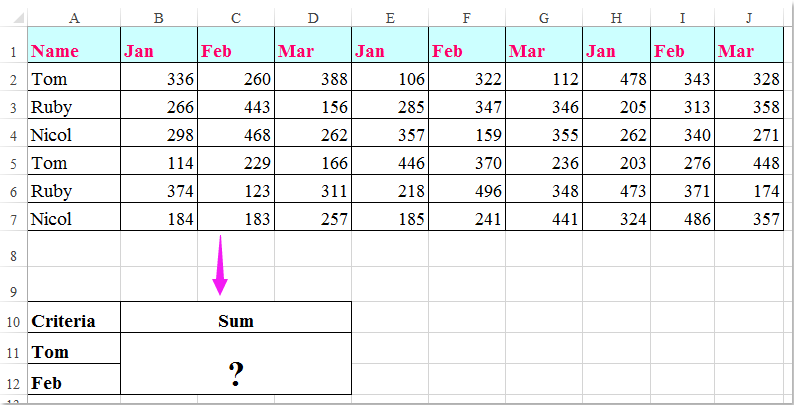
Mám řadu dat, která obsahuje záhlaví řádků a sloupců, teď chci vzít součet buněk, které splňují kritéria záhlaví sloupců i řádků. Chcete-li například sečíst buňky, jejichž kritériem sloupce je Tom a kritéria řádku, je únor, jak je znázorněno na následujícím obrázku. V tomto článku budu hovořit o některých užitečných vzorcích, jak to vyřešit.

kritéria řádku sloupce součtu dokumentu 1

Součet buněk na základě kritérií sloupců a řádků pomocí vzorců


šipka modrá pravá bublina Součet buněk na základě kritérií sloupců a řádků pomocí vzorců

Zde můžete použít následující vzorce k sečtení buněk na základě kritérií sloupců i řádků, postupujte takto:

Zadejte libovolný z níže uvedených vzorců do prázdné buňky, do které chcete výsledek odeslat:

=SUMPRODUCT((A2:A7="Tom")*(B1:J1="Feb")*(B2:J7))

=SUM(IF(B1:J1="Feb",IF(A2:A7="Tom",B2:J7)))

A pak stiskněte Shift + Ctrl + Enter společně získáte výsledek, viz screenshot:

kritéria řádku sloupce součtu dokumentu 2

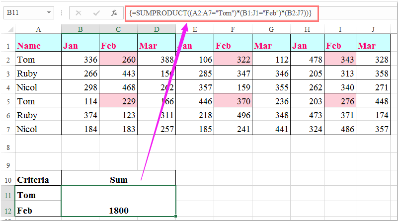
Poznámka: Ve výše uvedených vzorcích: Tomáš a února jsou kritéria sloupců a řádků, na základě A2: A7, B1: J1 jsou záhlaví sloupců a záhlaví řádků obsahují kritéria, B2: J7 je rozsah dat, který chcete sečíst.

Nejlepší nástroje pro produktivitu v kanceláři

🤖 Kutools AI asistent: Revoluční analýza dat založená na: Inteligentní provedení   |  Generovat kód  |  Vytvořte vlastní vzorce  |  Analyzujte data a generujte grafy  |  Vyvolejte funkce Kutools...
Populární funkce: Najít, zvýraznit nebo identifikovat duplikáty   |  Odstranit prázdné řádky   |  Kombinujte sloupce nebo buňky bez ztráty dat   |   Kolo bez vzorce ...
Super vyhledávání: Více kritérií VLookup    VLookup s více hodnotami  |   VLookup na více listech   |   Fuzzy vyhledávání ....
Pokročilý rozevírací seznam: Rychle vytvořte rozevírací seznam   |  Závislý rozbalovací seznam   |  Vícenásobný výběr rozevíracího seznamu ....
Správce sloupců: Přidejte konkrétní počet sloupců  |  Přesunout sloupce  |  Přepnout stav viditelnosti skrytých sloupců  |  Porovnejte rozsahy a sloupce ...
Doporučené funkce: Zaměření mřížky   |  Návrhové zobrazení   |   Velký Formula Bar    Správce sešitů a listů   |  Knihovna zdrojů (Automatický text)   |  Výběr data   |  Zkombinujte pracovní listy   |  Šifrovat/dešifrovat buňky    Odesílat e-maily podle seznamu   |  Super filtr   |   Speciální filtr (filtr tučné/kurzíva/přeškrtnuté...) ...
Top 15 sad nástrojů12 Text Tools (doplnit text, Odebrat znaky, ...)   |   50+ Graf Typ nemovitosti (Ganttův diagram, ...)   |   40+ Praktické Vzorce (Vypočítejte věk na základě narozenin, ...)   |   19 Vložení Tools (Vložte QR kód, Vložit obrázek z cesty, ...)   |   12 Konverze Tools (Čísla na slova, Přepočet měny, ...)   |   7 Sloučit a rozdělit Tools (Pokročilé kombinování řádků, Rozdělit buňky, ...)   |   ... a více

Rozšiřte své dovednosti Excel pomocí Kutools pro Excel a zažijte efektivitu jako nikdy předtím. Kutools for Excel nabízí více než 300 pokročilých funkcí pro zvýšení produktivity a úsporu času.  Kliknutím sem získáte funkci, kterou nejvíce potřebujete...

Popis


Office Tab přináší do Office rozhraní s kartami a usnadňuje vám práci

  • Povolte úpravy a čtení na kartách ve Wordu, Excelu, PowerPointu, Publisher, Access, Visio a Project.
  • Otevřete a vytvořte více dokumentů na nových kartách ve stejném okně, nikoli v nových oknech.
  • Zvyšuje vaši produktivitu o 50%a snižuje stovky kliknutí myší každý den!
Comments (17)
No ratings yet. Be the first to rate!
This comment was minimized by the moderator on the site
Brilliant!

The function =SUM(IF(B1:J1="Feb",IF(A2:A7="Tom",B2:J7))) is a great X & Y summation tool.
I would not have thought this logic out on my own.
In fact i took me a minute to deconstruction the operations.

Thank you
This comment was minimized by the moderator on the site
My data that I am trying to retrieve is in a table. Would this impact the result at all? I have:

=SUM(IF('[Primary Controller Active Project Database (KC notes)1.xlsx]Active Project Tracking'!$B2:$B66=X2,IF('[Primary Controller Active Project Database (KC notes)1.xlsx]Active Project Tracking'!$A1:$AV1=AH10,'[Primary Controller Active Project Database (KC notes)1.xlsx]Active Project Tracking'!$H$2:$AV$66)))

So I think the equivalent would be if you did your information above, but in a table in a different workbook. Thoughts?
This comment was minimized by the moderator on the site
If there were negatives in the matrix and you only wanted to include the positives, what would you do? 
I tried to do something like this:

=SUMPRODUCT((Column = Criteria)* ( Row = Criteria) * (second column = Criteria) * (Matrix) * (Matrix >0))

This comment was minimized by the moderator on the site
Is there a way to do this but instead of writing "Tom" & "Feb" in the formula, you are able to reference the criteria cells e.g.A11 & A12?
This comment was minimized by the moderator on the site
Hello, Rianna,Yest, as you said, you can use the cell references to replace the text in the formula, such as:
=SUMPRODUCT((A2:A7=A2)*(B1:J1=C1)*(B2:J7))
=SUM(IF(B1:J1=C1,IF(A2:A7=A2,B2:J7)))
This comment was minimized by the moderator on the site
In the above example which formula should I use if I wanted calculate the sum of the amounts earned by Tom Ruby & Nicol in March?
This comment was minimized by the moderator on the site
Hello, Nabar,To get the result you want, please apply the below formula:=SUMPRODUCT(((A2:A7="Tom")+(A2:A7="Nicol")+(A2:A7="Ruby"))*(B1:J1="Mar")*(B2:J7))
Please try, hope it can help you!
This comment was minimized by the moderator on the site
Hello Skyyang,
Thank you for your response. I tried the formula you suggested but I am not getting the right answer. Probably I wasn't able to put my query correctly. Let me try again I have a spreadsheet with data with daily calculation, I have numbered the first row 1,2,3,4.....132. 2nd, 3rd 4th &5th rows has table headings. The first column has line no's numbered 1, 2,3,.....3005 starting from row 6,range B6:EF3005 has data filled in on everyday basis. In second sheet i have a table in which I want to apply a formula which will look up two line numbers fed in two different rows and calculate the sum from the range B6: EF3005 from the data spreadsheet between the two line numbers from a certain column viz sum of values in column 15 between rows (line No's) 50 & 85.
This comment was minimized by the moderator on the site
Is there a way to make this work with wildcard characters? I'd like to use it on everything starting with certain characters, but with (a fixed number of) undefined characters at the end, i.e. =SUM(IF(B1:J1="Fe*",IF(A2:A7="To*",B2:J7)))
This comment was minimized by the moderator on the site
Should anyone have the same question, this is how I solved it (in Google Sheets, not tested in Excel):

=ArrayFormula(SUM(IF(regexmatch(O5:W5,"^Fe."),IF(regexmatch(N6:N11,"^To."),O6:W11))))

Note that the IF function does not support wildcard characters and that for regexmatch the wildcards are different and can be found here: https://github.com/google/re2/blob/master/doc/syntax.txt
In this particular instance, I used ^ to indicate that Fe & Tom occur at the beginning of text and . to allow for any following character (* would mean zero or more of the previous character, e.g. Fe* would only look for instances with 1 or more "e"s after F)
This comment was minimized by the moderator on the site
I tried to create a formula to calculate if the D12 is blank, it will calculate from K12 to AH12 but it seems this part ' regexmatch(D12,"")' is not working
ArrayFormula(SUM(IF(regexmatch(D12,""),K12:AH12)))
This comment was minimized by the moderator on the site
Thank you so much! You made my day!! @TeSageDS
This comment was minimized by the moderator on the site
how would you do this same formula if you wanted to sum both Feb and March together? please help! thanks

=SUMPRODUCT((A2:A7="Tom")*(B1:J1="Feb")*(B2:J7))
This comment was minimized by the moderator on the site
Hello,Angela,
To solve your problem, you just need to apply the below formula, please try it.

=SUMPRODUCT((A2:A7="Tom")*((B1:J1="Feb")+(B1:J1="Mar"))*(B2:J7)).

Hope it can help you!
This comment was minimized by the moderator on the site
Brilliant
This comment was minimized by the moderator on the site
Worth pointing out that of the two formulas provided above you do not need to enter the SUMPRODUCT formula with Ctrl + Shift + Enter. It will work perfectly well without it.
This comment was minimized by the moderator on the site
Awesome, this is the one what i was looking for. thanks for the help
There are no comments posted here yet
Please leave your comments in English
Posting as Guest
×
Rate this post:
0   Characters
Suggested Locations