Přejít k hlavnímu obsahu

Jak vytvořit vlastní vyhledávací pole v aplikaci Excel?

Kromě použití funkce Najít v aplikaci Excel můžete ve skutečnosti vytvořit vlastní vyhledávací pole pro snadné vyhledávání potřebných hodnot. Tento článek vám podrobně představí dvě metody, jak vytvořit vlastní vyhledávací pole v aplikaci Excel.

Vytvořte si vlastní vyhledávací pole s podmíněným formátováním, které zvýrazní všechny hledané výsledky
Vytvořte si vlastní vyhledávací pole se vzorci pro výpis všech hledaných výsledků


Vytvořte si vlastní vyhledávací pole s podmíněným formátováním, které zvýrazní všechny hledané výsledky

Chcete-li vytvořit vlastní vyhledávací pole pomocí funkce Podmíněné formátování v aplikaci Excel, můžete postupovat následovně.

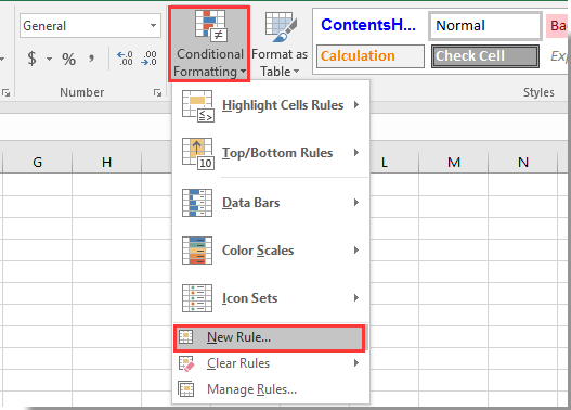
1. Do vyhledávacího pole vyberte rozsah s daty, která potřebujete prohledat, a poté klepněte na Podmíněné formátování > Nové pravidlo pod Domů záložka. Viz snímek obrazovky:

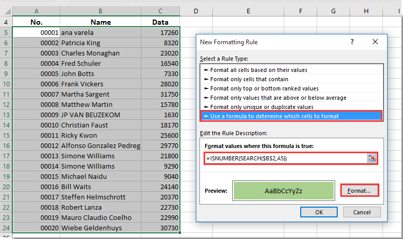
2. V Nové pravidlo pro formátování dialogové okno, musíte:

2.1) Vyberte Pomocí vzorce určete, které buňky chcete formátovat možnost v Vyberte typ pravidla krabice;

2.2) Zadejte vzorec = ISNUMBER (SEARCH ($ B $ 2, A5)) do Formátovat hodnoty, kde je tento vzorec pravdivý krabice;

2.3) Klikněte na Formát tlačítko pro určení zvýrazněné barvy pro hledanou hodnotu;

2.4) Klikněte na OK .

Poznámky:

1. Ve vzorci je $ B $ 2 prázdná buňka, kterou musíte použít jako vyhledávací pole, a A5 je první buňka ve vybraném rozsahu, ve kterém musíte hledat hodnoty. Změňte je prosím podle potřeby.

2. Vzorec nerozlišuje velká a malá písmena.

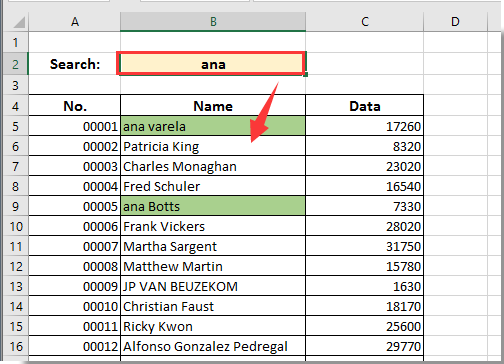
Nyní je vytvořeno vyhledávací pole, když zadáte vyhledávací kritéria do vyhledávacího pole B2 a stisknete klávesu Enter, budou vyhledány všechny odpovídající hodnoty v zadaném rozsahu a okamžitě zvýrazněny, jak je uvedeno níže.


Vytvořte si vlastní vyhledávací pole se vzorci pro výpis všech hledaných výsledků

Předpokládejme, že máte seznam dat v rozsahu E4: E23, který potřebujete vyhledat, pokud chcete po vyhledání pomocí vlastního vyhledávacího pole zobrazit všechny shodné hodnoty v jiném sloupci, můžete zkusit níže uvedenou metodu.

1. Vyberte prázdnou buňku sousedící s buňkou E4, zde vyberu buňku D4 a poté zadejte vzorec = IFERROR (SEARCH ($ B $ 2, E4) + ROW () / 100000, "") do řádku vzorců a poté stiskněte vstoupit klíč. Viz snímek obrazovky:

Poznámka: Ve vzorci je $ B $ 2 buňka, kterou potřebujete použít jako vyhledávací pole, E4 je první buňka seznamu dat, kterou potřebujete prohledat. Můžete je změnit, jak potřebujete.

2. Pokračujte ve výběru buňky E4 a potom přetáhněte rukojeť výplně dolů do buňky D23. Viz screenshot:

3. Nyní vyberte buňku C4, zadejte vzorec = IFERROR (RANK (D4, $ D $ 4: $ D $ 23,1), "") do řádku vzorců a stiskněte vstoupit klíč. Vyberte buňku C4 a poté přetáhněte rukojeť výplně dolů na C23. Viz screenshot:

4. Nyní musíte vyplnit rozsah A4: A23 číslem série, které se zvyšuje o 1 z 1 na 20, jak je uvedeno níže:

5. Vyberte prázdnou buňku, kterou potřebujete k zobrazení výsledku hledání, zadejte vzorec = IFERROR (VLOOKUP (A4, $ C $ 4: $ E $ 23,3, FALSE), "") do řádku vzorců a stiskněte vstoupit klíč. Pokračujte ve výběru buňky B4, přetáhněte rukojeť výplně dolů na B23, jak je uvedeno níže.

Od této chvíle budou při zadávání dat do vyhledávacího pole B2 všechny shodné hodnoty uvedeny v rozsahu B4: B23, jak je uvedeno níže.

Poznámka: tato metoda nerozlišuje velká a malá písmena.

Nejlepší nástroje pro produktivitu v kanceláři

🤖 Kutools AI asistent: Revoluční analýza dat založená na: Inteligentní provedení   |  Generovat kód  |  Vytvořte vlastní vzorce  |  Analyzujte data a generujte grafy  |  Vyvolejte funkce Kutools...
Populární funkce: Najít, zvýraznit nebo identifikovat duplikáty   |  Odstranit prázdné řádky   |  Kombinujte sloupce nebo buňky bez ztráty dat   |   Kolo bez vzorce ...
Super vyhledávání: Více kritérií VLookup    VLookup s více hodnotami  |   VLookup na více listech   |   Fuzzy vyhledávání ....
Pokročilý rozevírací seznam: Rychle vytvořte rozevírací seznam   |  Závislý rozbalovací seznam   |  Vícenásobný výběr rozevíracího seznamu ....
Správce sloupců: Přidejte konkrétní počet sloupců  |  Přesunout sloupce  |  Přepnout stav viditelnosti skrytých sloupců  |  Porovnejte rozsahy a sloupce ...
Doporučené funkce: Zaměření mřížky   |  Návrhové zobrazení   |   Velký Formula Bar    Správce sešitů a listů   |  Knihovna zdrojů (Automatický text)   |  Výběr data   |  Zkombinujte pracovní listy   |  Šifrovat/dešifrovat buňky    Odesílat e-maily podle seznamu   |  Super filtr   |   Speciální filtr (filtr tučné/kurzíva/přeškrtnuté...) ...
Top 15 sad nástrojů12 Text Tools (doplnit text, Odebrat znaky, ...)   |   50+ Graf Typ nemovitosti (Ganttův diagram, ...)   |   40+ Praktické Vzorce (Vypočítejte věk na základě narozenin, ...)   |   19 Vložení Tools (Vložte QR kód, Vložit obrázek z cesty, ...)   |   12 Konverze Tools (Čísla na slova, Přepočet měny, ...)   |   7 Sloučit a rozdělit Tools (Pokročilé kombinování řádků, Rozdělit buňky, ...)   |   ... a více

Rozšiřte své dovednosti Excel pomocí Kutools pro Excel a zažijte efektivitu jako nikdy předtím. Kutools for Excel nabízí více než 300 pokročilých funkcí pro zvýšení produktivity a úsporu času.  Kliknutím sem získáte funkci, kterou nejvíce potřebujete...

Popis


Office Tab přináší do Office rozhraní s kartami a usnadňuje vám práci

  • Povolte úpravy a čtení na kartách ve Wordu, Excelu, PowerPointu, Publisher, Access, Visio a Project.
  • Otevřete a vytvořte více dokumentů na nových kartách ve stejném okně, nikoli v nových oknech.
  • Zvyšuje vaši produktivitu o 50%a snižuje stovky kliknutí myší každý den!
Comments (29)
No ratings yet. Be the first to rate!
This comment was minimized by the moderator on the site
me pueden apoyar en cual es la formula para solo buscar
porfa
This comment was minimized by the moderator on the site
Hi, for the second part: "Create Your Own Search Box With Formulas To List All Searched Results", it doesn't say what to do with the search box, my search box has no formula in it. I am trying to do it with multiple columns as well, does it work too?
This comment was minimized by the moderator on the site
Insert data from example. Copy formula in indicated cell, but delete space from formula. Easy!
This comment was minimized by the moderator on the site
i have tried using this but is dose not wont to highlight the box I am searching for why is this
This comment was minimized by the moderator on the site
Can you create a formula that captures two cells worth of information in retrospect i am using a set up that captures user names and badge data so i need it to when it filters that it carries both cells of information not just one
This comment was minimized by the moderator on the site
hi! I used the basic highlight search bar, but am having a couple of issues. it is predicting my search and finding it with no issues... however, it always highlights the cell a couple below or above the searched one. Are you able to help me with this please?
This comment was minimized by the moderator on the site
Hi! Is this applicable to Google Sheets? I'm trying to make a search box with formulas to list all searched results. I followed every steps listed above but the results shows nothing. There is an error tho, it says "change Iterative calculation". But whatever I do, it doesn't show anything - just blank. Can you help me with this, please... Thank you!
This comment was minimized by the moderator on the site
Good day,
This is only applicable to Microsoft Excel application. Sorry for the inconvenience.
This comment was minimized by the moderator on the site
Hi! Is this applicable to Google Sheets? I'm trying to make a search box with formulas to list all searched results. I followed every steps listed above but the results shows nothing. There is an error tho, it says "change Iterative calculation". But whatever I do, it doesn't show anything - just blank. Can you help me with this, please... Thank you!
This comment was minimized by the moderator on the site
Hello, I am using to search between my vendors (one column) and brands (another column). With this setup, there are brands (like Microsoft) that can have more vendors (vendor A, vendor B, vendor C,...). I would like to search for the brand (microsoft) name and would like to see all possible vendors (A, B & C as well). But now the result is only the first vendor and that's all. How can I change/fix that?

Many thanks!
This comment was minimized by the moderator on the site
Hi Tomas,
Maybe you can rearrange your data and create a dynamic drop down list to solve the problem. You can browse the below article for more details.
https://www.extendoffice.com/documents/excel/1350-excel-create-dynamic-drop-down-list.html
This comment was minimized by the moderator on the site
i followed the resulted search method and it worked perfectly however the results are hyperlinked and it shows me the result without the hyperlink is there a way i can make it show me the result with the link connection?
This comment was minimized by the moderator on the site
After entering the formula =ISNUMBER(SEARCH($B$1,A4)) for conditional formatting, if the cell I used for the search function is blank, all the cells that are searched (A4:C368) are highlighted. But once a string is entered for the search criteria the cells containing the search criteria are highlighted correctly. Is there a way to tweak the formula to not highlight until search criteria is entered? Or did I do something wrong?

Also, using the formula in step 5 on another sheet within the workbook isn't working. What I'm trying to do is perform a search and show results of that search on one sheet named Search & Results while having the information to be searched on a sheet named Index. The formula I'm using is =IFERROR(VLOOKUP(A3,Index!$A$4:$C$368,5,FALSE),"") where A3 is the beginning of my numbered cells on the Search & Results sheet and the search is taking place throughout cells A4:C368 on the Index sheet.
This comment was minimized by the moderator on the site
same had been having the same issue with the formula,try this in your conditional formatting rule "=AND($I$1<>"",ISNUMBER(SEARCH($I$1,$B4)))", it works for me
I1 is my search box, B4 is first cell of selected range
This comment was minimized by the moderator on the site
Hi Colby. Your vlookup formula=IFERROR(VLOOKUP(A3,Index!$A$4:$C$368,5,FALSE),"") refers to range from A4 to C368 in Sheet name index which have only 3 column but you are entering 5 right after $C$368 which tells the vlookup formula to display value of column 5 which does not exists in your selected range. Fix this and I believe that your problem will be solved.
This comment was minimized by the moderator on the site
I have the same problem. Did you get an answer?
This comment was minimized by the moderator on the site
also me. i have the same problem
There are no comments posted here yet
Load More
Please leave your comments in English
Posting as Guest
×
Rate this post:
0   Characters
Suggested Locations