Přejít k hlavnímu obsahu

Jak podmíněné formátování na základě jiného listu v listu Google?

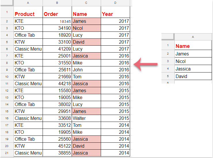
Pokud chcete použít podmíněné formátování na zvýraznění buněk na základě seznamu dat z jiného listu, jak ukazuje následující snímek obrazovky zobrazený v listu Google, máte nějaké jednoduché a dobré metody pro jeho řešení?

Podmíněné formátování pro zvýraznění buněk na základě seznamu z jiného listu v Tabulkách Google


Podmíněné formátování pro zvýraznění buněk na základě seznamu z jiného listu v Tabulkách Google


K dokončení této úlohy proveďte následující kroky:

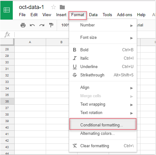
1, klikněte Formát > Podmíněné formátování, viz screenshot:

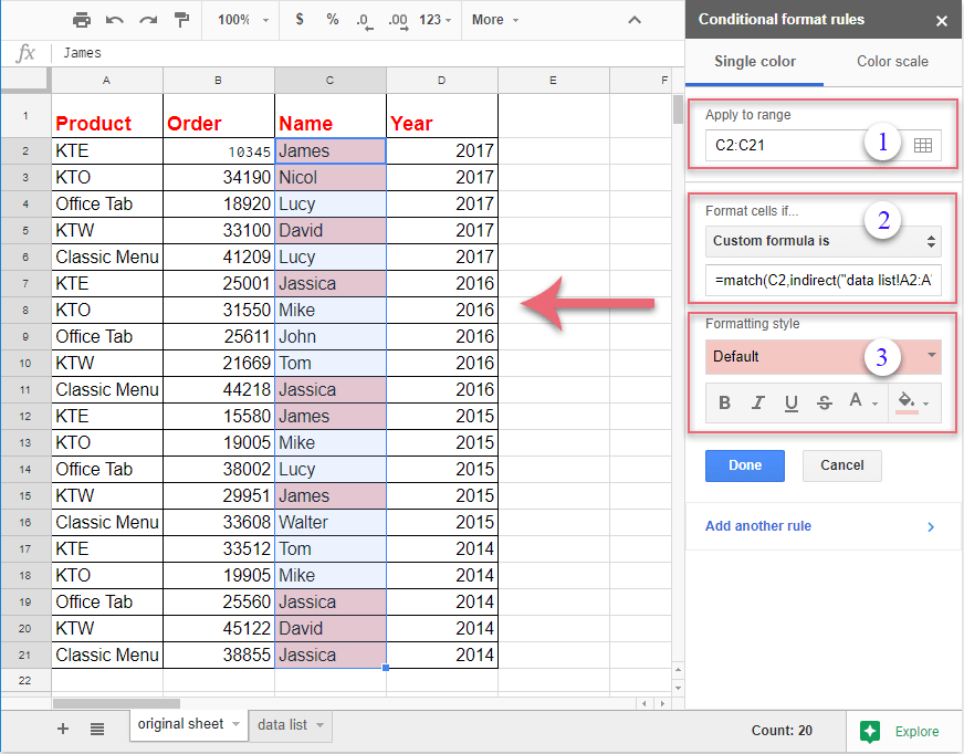
2. V Pravidla podmíněného formátu v podokně proveďte následující operace:

(1.) Klikněte tlačítko pro výběr dat sloupce, který chcete zvýraznit;

(2.) V Naformátujte buňky, pokud rozevírací seznam, prosím vyberte Vlastní vzorec je možnost a poté zadejte tento vzorec: = shoda (C2, nepřímý ("seznam dat! A2: A"), 0) do textového pole;

(3.) Poté vyberte jedno formátování z Formátování stylu jak potřebujete.

Poznámka: Ve výše uvedeném vzorci: C2 je první buňka dat sloupce, kterou chcete zvýraznit, a seznam dat! A2: A je rozsah listu a seznamu buněk, který obsahuje kritéria, podle kterých chcete buňky zvýraznit.

3. A všechny odpovídající buňky založené na buňkách seznamu byly zvýrazněny najednou, pak byste měli kliknout na Hotovo pro zavření Pravidla podmíněného formátu podokno, jak potřebujete.


Nejlepší nástroje pro produktivitu v kanceláři

🤖 Kutools AI asistent: Revoluční analýza dat založená na: Inteligentní provedení   |  Generovat kód  |  Vytvořte vlastní vzorce  |  Analyzujte data a generujte grafy  |  Vyvolejte funkce Kutools...
Populární funkce: Najít, zvýraznit nebo identifikovat duplikáty   |  Odstranit prázdné řádky   |  Kombinujte sloupce nebo buňky bez ztráty dat   |   Kolo bez vzorce ...
Super vyhledávání: Více kritérií VLookup    VLookup s více hodnotami  |   VLookup na více listech   |   Fuzzy vyhledávání ....
Pokročilý rozevírací seznam: Rychle vytvořte rozevírací seznam   |  Závislý rozbalovací seznam   |  Vícenásobný výběr rozevíracího seznamu ....
Správce sloupců: Přidejte konkrétní počet sloupců  |  Přesunout sloupce  |  Přepnout stav viditelnosti skrytých sloupců  |  Porovnejte rozsahy a sloupce ...
Doporučené funkce: Zaměření mřížky   |  Návrhové zobrazení   |   Velký Formula Bar    Správce sešitů a listů   |  Knihovna zdrojů (Automatický text)   |  Výběr data   |  Zkombinujte pracovní listy   |  Šifrovat/dešifrovat buňky    Odesílat e-maily podle seznamu   |  Super filtr   |   Speciální filtr (filtr tučné/kurzíva/přeškrtnuté...) ...
Top 15 sad nástrojů12 Text Tools (doplnit text, Odebrat znaky, ...)   |   50+ Graf Typ nemovitosti (Ganttův diagram, ...)   |   40+ Praktické Vzorce (Vypočítejte věk na základě narozenin, ...)   |   19 Vložení Tools (Vložte QR kód, Vložit obrázek z cesty, ...)   |   12 Konverze Tools (Čísla na slova, Přepočet měny, ...)   |   7 Sloučit a rozdělit Tools (Pokročilé kombinování řádků, Rozdělit buňky, ...)   |   ... a více

Rozšiřte své dovednosti Excel pomocí Kutools pro Excel a zažijte efektivitu jako nikdy předtím. Kutools for Excel nabízí více než 300 pokročilých funkcí pro zvýšení produktivity a úsporu času.  Kliknutím sem získáte funkci, kterou nejvíce potřebujete...

Popis


Office Tab přináší do Office rozhraní s kartami a usnadňuje vám práci

  • Povolte úpravy a čtení na kartách ve Wordu, Excelu, PowerPointu, Publisher, Access, Visio a Project.
  • Otevřete a vytvořte více dokumentů na nových kartách ve stejném okně, nikoli v nových oknech.
  • Zvyšuje vaši produktivitu o 50%a snižuje stovky kliknutí myší každý den!


Comments (27)
Rated 5 out of 5 · 2 ratings
This comment was minimized by the moderator on the site
Hi! skyyang ! Thank you, =match(C2,indirect("data list!A2:A"),0) works for me.

But I would like to format more than one column, so column A in sheet a is checked against column B in sheet b , and so.
There are so many columns so I can not apply one format per column, but a whole conditional format for the whole sheet.


How should I modify the range and the formula?

Thanks!
This comment was minimized by the moderator on the site
What if the cell values you're trying to match are hyperlinks?
Rated 5 out of 5
This comment was minimized by the moderator on the site
Pardon, il fallait lire =A1<>INDIRECT("PreviousVersion!"& CHAR (COLUMN () + 64) & ROW ()) ...
This comment was minimized by the moderator on the site
Bonjour,
J'ai une autre question du même type au sujet d'un formatage conditionnel qui fonctionne sur Excel mais que je n'arrive pas à porter sur Google Sheet :
L'idée est de comparer 2 versions d'une même feuille que l'on stock à l'aide de 2 onglets (2 feuilles du même workbook)

La formule est la suivante : =A1<>'previousVersion'!A1 avec un formatage fond jaune pour mettre en évidence les changements sur toute la feuille car l'idée est d'appliquer ce
formatage conditionnel sur toutes les cellules de la feuille ($A$1:$V:1000)

Sur Google sheet cette formule m'est interdite et si je passe par un "indirect("previousVersion!A1"), je perds le coté dynamique sur le "A1" de la feuille precious version
Si j'essaye =A1<>indirect("previousVersion!"&A1) j'ai une erreur car c'est la valeur de A1 qui est interprétée et concaténée avec "previousVersion!"

Si j'essaye la formule =C3<>INDIRECT("PreviousVersion!"& CHAR (COLUMN () + 64) & ROW ()) cela ne fonctionne pas non plus....

Si vous avez une solution...
Merci d'avance
This comment was minimized by the moderator on the site
Bonjour,
Dans Feuille google je cherche la formule suivante
Si dans la cel A1 = text alors dans la Cel B1 ecire telle valeur ou texte automatiquement
Merci d avance pour votre aide
This comment was minimized by the moderator on the site
What if it's not an exact match but contains the reference data.
This comment was minimized by the moderator on the site
Hello, ashley
To solve your problem, please apply the below formula:
=REGEXMATCH(C2:C21,INDIRECT("Sheet2!$A$2"))

Please try, hope it can help you!
This comment was minimized by the moderator on the site
What happens if the data in my list is in more than one column? When I try to use datalist!A2:M or datalist!A:M or datalist!A2:M17 none of those work.
This comment was minimized by the moderator on the site
I have even tried naming the specific range I want to refer to and using that in the formula, no luck.
This comment was minimized by the moderator on the site
How to highlight the entire row data with conditional formatting using other sub-sheet
This comment was minimized by the moderator on the site
Hello, Ranganath
To highlight the entire row based on the data list, please do as this:
1. In the Apply to range box, select the whole sheet;
2. Apply this formula: =match($C2,indirect("datalist!A2:A"),0) into the Custom formula is textbox.
Please try, hope it can help you!

https://www.extendoffice.com/images/stories/comments/comment-skyyang/doc-highlight-entire-row.png
This comment was minimized by the moderator on the site
Hey, Thanks for replying. I have tried the formula but its not working.
Rated 5 out of 5
This comment was minimized by the moderator on the site
Hi,
Have you modified the sheet name and cell reference to your own data?
$C2 is the first cell of the column data that you want to highlight, and the datalist!A2:A is another sheet name and list range which contains the criteria you want to highlight the cells based on.
Please check them, thank you!
This comment was minimized by the moderator on the site
This doesn't work for me. I have triple checked everything.

Apply to range: K1:K2158

=match(K2,indirect("TorontoCitys!A1:A"),0)

It highlights random other city names, not in the TorontoCity's list.

K2 (is my main sheet and the starting column cell of the column I want to be affected.
TorontoCitys (is the name of the sheet)
A1 is the start of the column of the list of city names.
A is the column.

Could be that my punctuation's are incorrect?

Thanks in advance.
This comment was minimized by the moderator on the site
Hello friend,

Glad to help. Your formula is correct, please don't worry. The problem is the range you apply to. It shouldn't be K1:K2158, but K2:K2158.

Please see the screenshots. The example is simple but enough to explain the problem.

The correct "Apply to Range" is A2:A20. And the correct formula is =match(A2,indirect("TorontoCitys!A1:A"),0). Then correct cities can be highlighted. Please see screenshot 2.
But if I change the "Apply to Range" to A1:A20, the wrong city name is highlighted. Please see screenshot 3.

So please change your "Apply to Range" from K1:K2158 to K2:K2158. The problem should be solved. Looking forward to your reply.

Sincerely,
Mandy
This comment was minimized by the moderator on the site
how do you do this but with the entire row highlighted
There are no comments posted here yet
Load More
Please leave your comments in English
Posting as Guest
×
Rate this post:
0   Characters
Suggested Locations