Jak sčítat buňky, pokud obsahuje část textového řetězce v goolge listech?
Chcete-li sečíst hodnoty buněk ve sloupci, pokud jiné buňky sloupce obsahují část konkrétního textového řetězce, jak ukazuje následující snímek obrazovky, tento článek představí užitečný vzorec pro řešení tohoto úkolu v tabulkách Google.
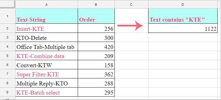
Buňky sumif, pokud obsahuje část konkrétního textového řetězce v tabulkách Google se vzorci
Buňky sumif, pokud obsahuje část konkrétního textového řetězce v tabulkách Google se vzorci
Následující vzorce vám pomohou sečíst hodnoty buněk, pokud jiné buňky sloupců obsahují konkrétní textový řetězec, postupujte takto:
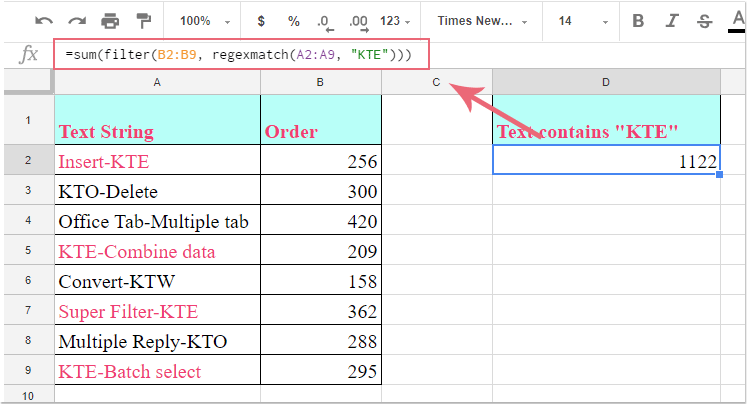
1. Zadejte tento vzorec: =sum(filter(B2:B9, regexmatch(A2:A9, "KTE"))) do prázdné buňky a poté stiskněte vstoupit klíč k získání výsledku, viz screenshot:
Poznámky:
1. Ve výše uvedeném vzorci: B2: B9 jsou hodnoty buněk, které chcete sečíst, A2: A9 je rozsah obsahuje konkrétní textový řetězec, “KTE„Je konkrétní text, podle kterého chcete shrnout, změňte je prosím podle svých potřeb.
2. Zde je další vzorec, který vám může pomoci: =sumif(A2:A9,"*KTE*",B2:B9).
Nejlepší nástroje pro produktivitu v kanceláři
Rozšiřte své dovednosti Excel pomocí Kutools pro Excel a zažijte efektivitu jako nikdy předtím. Kutools for Excel nabízí více než 300 pokročilých funkcí pro zvýšení produktivity a úsporu času. Kliknutím sem získáte funkci, kterou nejvíce potřebujete...
")
Office Tab přináší do Office rozhraní s kartami a usnadňuje vám práci
- Povolte úpravy a čtení na kartách ve Wordu, Excelu, PowerPointu, Publisher, Access, Visio a Project.
- Otevřete a vytvořte více dokumentů na nových kartách ve stejném okně, nikoli v nových oknech.
- Zvyšuje vaši produktivitu o 50%a snižuje stovky kliknutí myší každý den!
")