Přejít k hlavnímu obsahu

Jak propojit filtr kontingenční tabulky s určitou buňkou v aplikaci Excel?

Pokud chcete propojit filtr kontingenční tabulky s určitou buňkou a provést kontingenční tabulku filtrovanou na základě hodnoty buňky, může vám pomoci metoda v tomto článku.

Propojte filtr kontingenční tabulky s určitou buňkou pomocí kódu VBA


Propojte filtr kontingenční tabulky s určitou buňkou pomocí kódu VBA

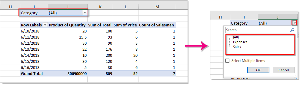
Kontingenční tabulka, kterou propojíte její funkci filtru s hodnotou buňky, by měla obsahovat pole filtru (název pole filtru hraje důležitou roli v následujícím kódu VBA).

Jako příklad si vezměte níže uvedenou kontingenční tabulku, volá se pole filtru v kontingenční tabulce Kategorie, a obsahuje dvě hodnoty „výdaje"A"Prodej“. Po propojení filtru kontingenční tabulky s buňkou by hodnoty buňky, které použijete pro filtrování kontingenční tabulky, měly být „Výdaje“ a „Prodej“.

1. Vyberte buňku (zde vyberu buňku H6), kterou propojíte s funkcí filtru kontingenční tabulky, a do buňky předem zadejte jednu z hodnot filtru.

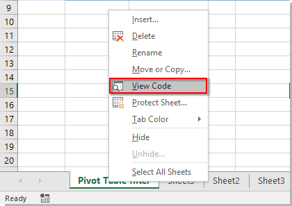
2. Otevřete list obsahující kontingenční tabulku, kterou propojíte s buňkou. Klikněte pravým tlačítkem na kartu listu a vyberte Zobrazit kód z kontextové nabídky. Viz snímek obrazovky:

3. V Microsoft Visual Basic pro aplikace zkopírujte níže uvedený kód VBA do okna Kód.

Kód VBA: Propojte filtr kontingenční tabulky s určitou buňkou

Private Sub Worksheet_Change(ByVal Target As Range)
'Update by Extendoffice 20180702
    Dim xPTable As PivotTable
    Dim xPFile As PivotField
    Dim xStr As String
    On Error Resume Next
    If Intersect(Target, Range("H6")) Is Nothing Then Exit Sub
    Application.ScreenUpdating = False
    Set xPTable = Worksheets("Sheet1").PivotTables("PivotTable2")
    Set xPFile = xPTable.PivotFields("Category")
    xStr = Target.Text
    xPFile.ClearAllFilters
    xPFile.CurrentPage = xStr
    Application.ScreenUpdating = True
End Sub

Poznámky:

1) "Sheet1„Je název otevřeného listu.
2) "Kontingenční tabulka 2„Je název kontingenční tabulky, kterou propojíte s funkcí filtru do buňky.
3) Filtrační pole v kontingenční tabulce se nazývá „Kategorie".
4) Odkazovaná buňka je H6. Tyto hodnoty proměnných můžete změnit podle svých potřeb.

4. zmáčkni Další + Q klávesy pro zavření Microsoft Visual Basic pro aplikace okno.

Nyní je funkce filtru kontingenční tabulky propojena s buňkou H6.

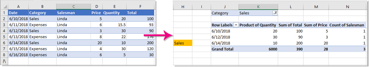
Obnovte buňku H6, poté se odpovídající data v kontingenční tabulce odfiltrují na základě existující hodnoty. Viz screenshot:

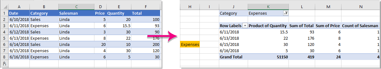
Při změně hodnoty buňky se filtrovaná data v kontingenční tabulce automaticky změní. Viz screenshot:


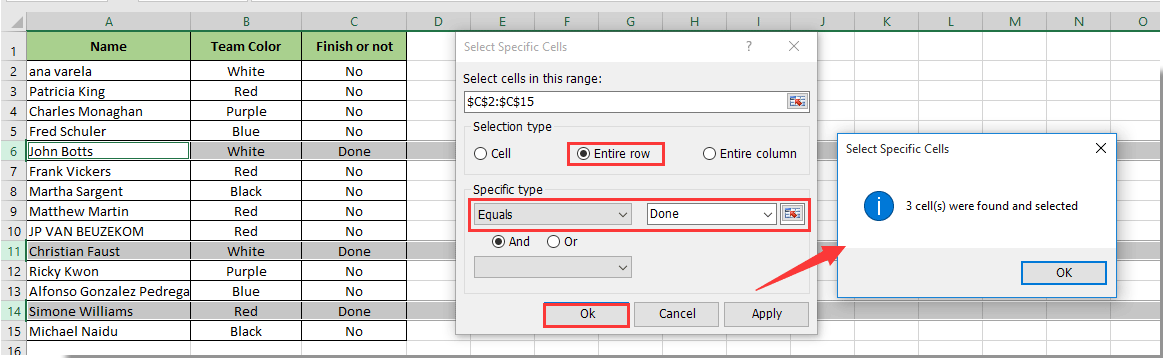
Snadno vyberte celé řádky na základě hodnoty buňky ve sloupci Certian:

Projekt Vyberte konkrétní buňky užitečnost Kutools pro Excel vám pomůže rychle vybrat celé řádky na základě hodnoty buňky ve sloupci certian v aplikaci Excel, jak je uvedeno níže. Po výběru všech řádků na základě hodnoty buňky je můžete ručně přesunout nebo zkopírovat do nového umístění podle potřeby v aplikaci Excel.
Stáhněte si a vyzkoušejte to hned! (30denní bezplatná trasa)


Související články:

Nejlepší nástroje pro produktivitu v kanceláři

🤖 Kutools AI asistent: Revoluční analýza dat založená na: Inteligentní provedení   |  Generovat kód  |  Vytvořte vlastní vzorce  |  Analyzujte data a generujte grafy  |  Vyvolejte funkce Kutools...
Populární funkce: Najít, zvýraznit nebo identifikovat duplikáty   |  Odstranit prázdné řádky   |  Kombinujte sloupce nebo buňky bez ztráty dat   |   Kolo bez vzorce ...
Super vyhledávání: Více kritérií VLookup    VLookup s více hodnotami  |   VLookup na více listech   |   Fuzzy vyhledávání ....
Pokročilý rozevírací seznam: Rychle vytvořte rozevírací seznam   |  Závislý rozbalovací seznam   |  Vícenásobný výběr rozevíracího seznamu ....
Správce sloupců: Přidejte konkrétní počet sloupců  |  Přesunout sloupce  |  Přepnout stav viditelnosti skrytých sloupců  |  Porovnejte rozsahy a sloupce ...
Doporučené funkce: Zaměření mřížky   |  Návrhové zobrazení   |   Velký Formula Bar    Správce sešitů a listů   |  Knihovna zdrojů (Automatický text)   |  Výběr data   |  Zkombinujte pracovní listy   |  Šifrovat/dešifrovat buňky    Odesílat e-maily podle seznamu   |  Super filtr   |   Speciální filtr (filtr tučné/kurzíva/přeškrtnuté...) ...
Top 15 sad nástrojů12 Text Tools (doplnit text, Odebrat znaky, ...)   |   50+ Graf Typ nemovitosti (Ganttův diagram, ...)   |   40+ Praktické Vzorce (Vypočítejte věk na základě narozenin, ...)   |   19 Vložení Tools (Vložte QR kód, Vložit obrázek z cesty, ...)   |   12 Konverze Tools (Čísla na slova, Přepočet měny, ...)   |   7 Sloučit a rozdělit Tools (Pokročilé kombinování řádků, Rozdělit buňky, ...)   |   ... a více

Rozšiřte své dovednosti Excel pomocí Kutools pro Excel a zažijte efektivitu jako nikdy předtím. Kutools for Excel nabízí více než 300 pokročilých funkcí pro zvýšení produktivity a úsporu času.  Kliknutím sem získáte funkci, kterou nejvíce potřebujete...

Popis


Office Tab přináší do Office rozhraní s kartami a usnadňuje vám práci

  • Povolte úpravy a čtení na kartách ve Wordu, Excelu, PowerPointu, Publisher, Access, Visio a Project.
  • Otevřete a vytvořte více dokumentů na nových kartách ve stejném okně, nikoli v nových oknech.
  • Zvyšuje vaši produktivitu o 50%a snižuje stovky kliknutí myší každý den!
Comments (38)
No ratings yet. Be the first to rate!
This comment was minimized by the moderator on the site
Hi,
This code worked perfectly on the pivot table, but I also want to link a filter to a cell value on a Table. Is there code for this? Please help :)
This comment was minimized by the moderator on the site
if my column in pivot table is date this code not working, can some one help me please
This comment was minimized by the moderator on the site
Можно ли сослаться вместо ячейки H6 на ячейку на другом листе? как это сделать? подскажите пожалуйста.
This comment was minimized by the moderator on the site
Hi Алексей,

You don't need to modify the code, just add the VBA code to the worksheet of the cell you want to reference.
For example, if you want to filter a pivot table named "PivotTable1" in Sheet2 based on the value of cell H6 in Sheet3, please right click the Sheet3 worksheet tab, click View Code from the right-clicking menu, and then add the code to the Sheet3 (Code) window.
This comment was minimized by the moderator on the site
Как сделать чтобы сводная таблица применяла сразу 2 фильтра из 2хразных ячеек? а не 1 как в примере?
This comment was minimized by the moderator on the site
Hi Алексей,

Please check if the VBA code in this comment #38754 can help.
This comment was minimized by the moderator on the site
find these and change it in Array(),Intersect(), Worksheets(), PivotFields()

PivotTable1
PivotTable2
PivotTable3
PivotTable4
H1
SheetName
FieldName


Private Sub Worksheet_Change(ByVal Target As Range)
'Update by Extendoffice 20180702
    Dim xPTable As PivotTable
    Dim xPFile As PivotField
    Dim xPTabled As PivotTable
    Dim xPFiled As PivotField
    Dim xStr As String
    On Error Resume Next
    '리스트 만들기
    Dim listArray() As Variant
    listArray = Array("PivotTable1", "PivotTable2", "PivotTable3", "PivotTable4")
    If Intersect(Target, Range("H1")) Is Nothing Then Exit Sub
    Application.ScreenUpdating = False
    For i = 0 To UBound(listArray)
        Set xPTable = Worksheets("SheetName").PivotTables(listArray(i))
        Set xPFile = xPTable.PivotFields("FieldName")
        'MsgBox (listArray(i))
        xStr = Target.Text
        xPFile.ClearAllFilters
        xPFile.CurrentPage = xStr
    Next
        Application.ScreenUpdating = True
End Sub
This comment was minimized by the moderator on the site
Hello,

This code works perfectly. However I am not able to get the code to update the pivot table automatically. The target value for me is a formula (=DATE(D18,..,..)) which changes depending on what is selected at D18. For it to update the pivot table i have to double click the target cell and hit enter. Is there a way around it?

Thank you
This comment was minimized by the moderator on the site
Hello ST,
Suppose your target value is in H6 and it changes depending on the value in D18. To filter a pivot table based on this target value. The following VBA code can help. Please give it a try.
Private Sub Worksheet_Change(ByVal Target As Range)
'Updated by Extendoffice 2022/07/22
Dim xPTable As PivotTable
Dim xPFile As PivotField
Dim xStr As String
Dim xBoolean As Boolean
Dim xItsRG As Range
Dim xDDs As Range
Dim xDs As Range
On Error Resume Next

xBoolean = False
Set xRg = Range("h6")

Set xItsRG = Intersect(Target, xRg)
Set xDDs = Intersect(Target.DirectDependents, xRg)
Set xDs = Intersect(Target.Dependents, xRg)
If Not (xItsRG Is Nothing) Then
    xBoolean = True
ElseIf Not (xDDs Is Nothing) Then
    xBoolean = True
ElseIf Not (xDs Is Nothing) Then
    xBoolean = True
End If


If Not xBoolean Then Exit Sub

Application.ScreenUpdating = False
Set xPTable = Worksheets("Sheet1").PivotTables("Pivot Table 1")
Set xPFile = xPTable.PivotFields("Category")
xStr = Target.Text
xPFile.ClearAllFilters
xPFile.CurrentPage = xStr
Application.ScreenUpdating = True

End Sub
This comment was minimized by the moderator on the site
Hello Crysal,

I added a line on the code : Dim xRg As Range

The code doesn't automatically reset the dates when the target is changed. I have an excel file replicating what I am trying to do, I a not able to add attachments on this website though. D3 (target = DATE(A15,B15,C15)) has an equation linked to A15, B15 and C15. When any value on A15, B15 and C15 is changed the pivot table resets to no filter. Could you help me out on this?
This comment was minimized by the moderator on the site
Hi ST,
I don't quite understand what you mean. In your case, the value of target cell D3 is used to filter the pivot table. The formula in the target cell D3 references the values of cells A15, B15 and C15, which will change according to the values in the reference cells. When any value on A15, B15 and C15 is changed, the pivot table will be automatically filtered if the value in the target cell meets the filter conditions of the pivot table. If the value in the target cell does not meet the pivot table's filtering criteria, the pivot table will be automatically reset to no filtering.
This comment was minimized by the moderator on the site
I’m not sure if there is a way to share an excel file with you. If my target value, which is a date, changes according to changes in other cells. I have to double click on the target cell and hit enter (like you would after entering a formula in a cell) to update the pivot table
This comment was minimized by the moderator on the site
Hi Sagar T,
The code has been updated. Please give it a try. Thanks for your feedback.
Don't forget to change the names of the worksheet, pivot table and the filter in the code. Or you can download the following uploaded workbook for testing.

Private Sub Worksheet_Change(ByVal Target As Range)
'Updated by Extendoffice 20220805
Dim xPTable As PivotTable
Dim xPFile As PivotField
Dim xStr As String
Dim xBoolean As Boolean
Dim xItsRG As Range
Dim xDDs As Range
Dim xDs As Range
On Error Resume Next

xBoolean = False
Set xRg = Range("D3")

Set xItsRG = Intersect(Target, xRg)
Set xDDs = Intersect(Target.DirectDependents, xRg)
Set xDs = Intersect(Target.Dependents, xRg)
If Not (xItsRG Is Nothing) Then
    xBoolean = True
ElseIf Not (xDDs Is Nothing) Then
    xBoolean = True
ElseIf Not (xDs Is Nothing) Then
    xBoolean = True
End If


If Not xBoolean Then Exit Sub
xStr = Format(xRg.Text, "m/d/yyyy")
Application.ScreenUpdating = False
Set xPTable = Worksheets("Sheet2").PivotTables("PivotTable1")
Set xPFile = xPTable.PivotFields("Date")
xPFile.ClearAllFilters
xPFile.CurrentPage = xStr
Application.ScreenUpdating = True

End Sub
This comment was minimized by the moderator on the site
Hello,

The code works fine for me. However I am not able to get the pivot table to update the filter target automatically. The target in my case is a formula [DATE(D18,S14,C18)]. The code only works when I double click the target cell and hit enter.

Thank you
This comment was minimized by the moderator on the site
Hi Justin,

This has worked perfectly, however, I am wondering if this rule can be applied to multiple PivotTables within the same sheet?

Thanks,
James
This comment was minimized by the moderator on the site
Change Values in Array(), Worksheets() and Intersect()


**Find these and change it**
SheetName
E1
PivotTable1
PivotTable2
PivotTable3


Private Sub Worksheet_Change(ByVal Target As Range)
'Update by Extendoffice 20180702
Dim xPTable As PivotTable
Dim xPFile As PivotField

Dim xPTabled As PivotTable
Dim xPFiled As PivotField

Dim xStr As String


On Error Resume Next

'리스트 만들기
Dim listArray() As Variant
listArray = Array("PivotTable1", "PivotTable2", "PivotTable3")


If Intersect(Target, Range("E1")) Is Nothing Then Exit Sub
Application.ScreenUpdating = False

For i = 0 To UBound(listArray)

Set xPTable = Worksheets("SheetName").PivotTables(listArray(i))
Set xPFile = xPTable.PivotFields("Company_ID")

xStr = Target.Text
xPFile.ClearAllFilters
xPFile.CurrentPage = xStr


Next

Application.ScreenUpdating = True


End Sub
This comment was minimized by the moderator on the site
Hi James,

Yes this is possible, code I used for this is (4 pivots and 2 cell references):

Private Sub Worksheet_Change(ByVal Target As Range)
Dim I As Integer
Dim xFilterStr1, xFilterStr2, yFilterstr1, yfilterstr2 As String
On Error Resume Next
If Intersect(Target, Range("O26:P27")) Is Nothing Then Exit Sub

xFilterStr1 = Range("O26").Value
xFilterStr2 = Range("O27").Value
yFilterstr1 = Range("p26").Value
yfilterstr2 = Range("p27").Value
ActiveSheet.PivotTables("Order_Comp_B2C_Crea").PivotFields("Week Number"). _
ActiveSheet.PivotTables("Order_Comp_B2B_Crea").PivotFields("Week Number"). _
ActiveSheet.PivotTables("Order_Comp_B2C_Disp").PivotFields("Week Number"). _
ActiveSheet.PivotTables("Order_Comp_B2B_Disp").PivotFields("Week Number"). _
ClearAllFilters

If xFilterStr1 = "" And xFilterStr2 = "" And yFilterstr1 = "" And yfilterstr2 = "" Then Exit Sub
ActiveSheet.PivotTables("Order_Comp_B2C_Crea").PivotFields("Week Number"). _
ActiveSheet.PivotTables("Order_Comp_B2B_Crea").PivotFields("Week Number"). _
ActiveSheet.PivotTables("Order_Comp_B2C_Disp").PivotFields("Week Number"). _
ActiveSheet.PivotTables("Order_Comp_B2B_Disp").PivotFields("Week Number"). _
EnableMultiplePageItems = True

xCount = ActiveSheet.PivotTables("Order_Comp_B2C_Crea").PivotFields("Week Number").PivotItems.Count
xCount = ActiveSheet.PivotTables("Order_Comp_B2B_Crea").PivotFields("Week Number").PivotItems.Count
yCount = ActiveSheet.PivotTables("Order_Comp_B2C_Disp").PivotFields("Week Number").PivotItems.Count
yCount = ActiveSheet.PivotTables("Order_Comp_B2B_Disp").PivotFields("Week Number").PivotItems.Count

For I = 1 To xCount
If I <> xFilterStr1 And I <> xFilterStr2 Then
ActiveSheet.PivotTables("Order_Comp_B2C_Crea").PivotFields("Week Number").PivotItems(I).Visible = False
ActiveSheet.PivotTables("Order_Comp_B2B_Crea").PivotFields("Week Number").PivotItems(I).Visible = False
Else
ActiveSheet.PivotTables("Order_Comp_B2C_Crea").PivotFields("Week Number").PivotItems(I).Visible = True
ActiveSheet.PivotTables("Order_Comp_B2B_Crea").PivotFields("Week Number").PivotItems(I).Visible = True
End If
Next

For I = 1 To yCount
If I <> yFilterstr1 And I <> yfilterstr2 Then
ActiveSheet.PivotTables("Order_Comp_B2C_Disp").PivotFields("Week Number").PivotItems(I).Visible = False
ActiveSheet.PivotTables("Order_Comp_B2B_Disp").PivotFields("Week Number").PivotItems(I).Visible = False
Else
ActiveSheet.PivotTables("Order_Comp_B2C_Disp").PivotFields("Week Number").PivotItems(I).Visible = True
ActiveSheet.PivotTables("Order_Comp_B2B_Disp").PivotFields("Week Number").PivotItems(I).Visible = True
End If
Next

End Sub
This comment was minimized by the moderator on the site
I used it for a normal excell and it worked.But I could not use it for an olap worksheets. maybe I need to change it a little?
This comment was minimized by the moderator on the site
Hi maziaritib4 TIB,
The method is only avaliable for Microsoft Excel. Sorry for the inconvenience.
This comment was minimized by the moderator on the site
Hi,

Tried to get this working for the column filter but does not seem to work. Do I need an other code for that?

Thanks
This comment was minimized by the moderator on the site
Hi Justin,
Did you get any error prompt? I need to know more specific about your issue.
Before applying the code, don't forget to modify the "name of the sheet", "name of the pivot table", "name of the filter of pivot table" and the cell you want to filter the pivot table based on (see sceenshot).
https://www.extendoffice.com/images/stories/comments/comment-picture-zxm/4.png
This comment was minimized by the moderator on the site
Hi Crystal,

Thanks for your help. Issue is the function is not doing anything for some reason. Some clarification:

Pivot name: Order_Comp_B2C
Sheet Name: Calculation Sheet
Filter name: Week Number (I changed this name from what was "Dispatch Week No" in the data file)
Cell to change: O26 and O27 (this should go in range)

In this pivot, I am trying to get the filter changed for the columns, I have nothing in the filter area in the PivotTable Fields menu.

my code is:

Private Sub Worksheet_Change(ByVal Target As Range)
'Update by Extendoffice 20180702
Dim xPTable As PivotTable
Dim xPFile As PivotField
Dim xStr As String
On Error Resume Next
If Intersect(Target, Range("O26")) Is Nothing Then Exit Sub
Application.ScreenUpdating = False
Set xPTable = Worksheets("Calculation Sheet").PivotTables("Order_Comp_B2C")
Set xPFile = xPTable.PivotFields("Week Number")
xStr = Target.Text
xPFile.ClearAllFilters
xPFile.CurrentPage = xStr
Application.ScreenUpdating = True
End Sub

Thanks,

Justin
This comment was minimized by the moderator on the site
Hi Justin Teeuw,
I have changed the Pivot name, sheet name, filter name and cell to change to the conditions you mentioned above, and tried the VBA code you provided, it works well in my case. See the following GIF or the attached workbook.
Do you mind creating a new workbook and try the code again?
https://www.extendoffice.com/images/stories/comments/comment-picture-zxm/6.gif
This comment was minimized by the moderator on the site
Hi Crystal,

Attached a screenshot of the pivot, the red box is the filter I would like to change based on the cell value.

Preferably I would like to use a range of cells indicating multiple week numbers.

Thanks,

Justin
This comment was minimized by the moderator on the site
Hi Justin Teeuw,
Please try the following VBA code. Hope I can help.

Private Sub Worksheet_Change(ByVal Target As Range)
    'Update by Extendoffice 20220706
    Dim I As Integer
    Dim xFilterStr1, xFilterStr2 As String
    On Error Resume Next
    If Intersect(Target, Range("O26:O27")) Is Nothing Then Exit Sub
    'Application.ScreenUpdating = False
    
    xFilterStr1 = Range("O26").Value
    xFilterStr2 = Range("O27").Value
    ActiveSheet.PivotTables("Order_Comp_B2C").PivotFields("Week Number"). _
        ClearAllFilters
    If xFilterStr1 = "" And xFilterStr2 = "" Then Exit Sub
    ActiveSheet.PivotTables("Order_Comp_B2C").PivotFields("Week Number"). _
        EnableMultiplePageItems = True
    xCount = ActiveSheet.PivotTables("Order_Comp_B2C").PivotFields("Week Number").PivotItems.Count

    For I = 1 To xCount
        If I <> xFilterStr1 And I <> xFilterStr2 Then
            ActiveSheet.PivotTables("Order_Comp_B2C").PivotFields("Week Number").PivotItems(I).Visible = False
        Else
            ActiveSheet.PivotTables("Order_Comp_B2C").PivotFields("Week Number").PivotItems(I).Visible = True
        End If
    Next

    'Application.ScreenUpdating = True
End Sub
This comment was minimized by the moderator on the site
Hi Justin,
Sorry I didn't see the screenshot you attached on the page. Maybe there is some error on the page.
If you still need to solve the problem, email me via . Sorry for the inconvenience.
There are no comments posted here yet
Load More
Please leave your comments in English
Posting as Guest
×
Rate this post:
0   Characters
Suggested Locations