Přejít k hlavnímu obsahu

Jak vrátit více hodnot shody na základě jednoho nebo více kritérií v aplikaci Excel?

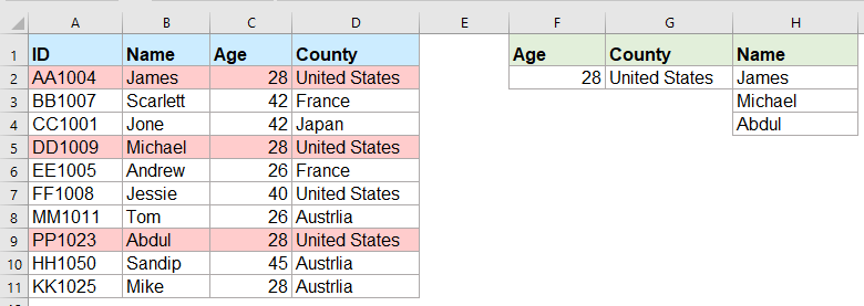
Za normálních okolností je vyhledání konkrétní hodnoty a vrácení odpovídající položky pro většinu z nás snadné pomocí funkce VLOOKUP. Ale pokusili jste se někdy vrátit více hodnot shody na základě jednoho nebo více kritérií, jak ukazuje následující snímek obrazovky? V tomto článku představím několik vzorců pro řešení tohoto složitého úkolu v aplikaci Excel.

Vraťte více shodných hodnot na základě jednoho nebo více kritérií s maticovými vzorci


Vraťte více shodných hodnot na základě jednoho nebo více kritérií s maticovými vzorci

Například chci extrahovat všechna jména, jejichž věk je 28 let a pocházejí ze Spojených států, použijte následující vzorec:

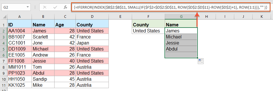
1. Zkopírujte nebo zadejte následující vzorec do prázdné buňky, kde chcete najít výsledek:

=INDEX($B$2:$B$11, SMALL(IF(COUNTIF($F$2, $C$2:$C$11)*COUNTIF($G$2, $D$2:$D$11), ROW($A$2:$D$11)-MIN(ROW($A$2:$D$11))+1), ROW(A1)), COLUMN(A1))

Poznámka: Ve výše uvedeném vzorci, B2: B11 je sloupec, ze kterého je vrácena odpovídající hodnota; F2, C2: C11 jsou první podmínka a data sloupce, která obsahuje první podmínku; G2, D2: D11 jsou druhá podmínka a data sloupce, která tuto podmínku obsahují, změňte je prosím podle potřeby.

2. Poté stiskněte tlačítko Ctrl + Shift + Enter klávesy pro získání prvního výsledku shody a poté vyberte první buňku vzorce a přetáhněte rukojeť výplně dolů do buněk, dokud se nezobrazí chybová hodnota, nyní se všechny odpovídající hodnoty vrátí, jak je znázorněno níže:

Tipy: Pokud potřebujete pouze vrátit všechny odpovídající hodnoty na základě jedné podmínky, použijte následující vzorec pole:

=IFERROR(INDEX($B$2:$B$11, SMALL(IF($F$2=$D$2:$D$11, ROW($D$2:$D$11)-ROW($D$2)+1), ROW(1:1))),"" )


Více relativních článků:

  • Vraťte více hodnot vyhledávání v jedné buňce oddělené čárkami
  • V aplikaci Excel můžeme použít funkci VLOOKUP k vrácení první shodné hodnoty z buněk tabulky, ale někdy musíme extrahovat všechny odpovídající hodnoty a poté je oddělit konkrétním oddělovačem, například čárkou, pomlčkou atd ... do jednoho buňka jako následující snímek obrazovky. Jak bychom mohli získat a vrátit více hodnot vyhledávání v jedné buňce oddělené čárkami v aplikaci Excel?
  • Vlookup a vrácení více odpovídajících hodnot najednou v tabulce Google
  • Normální funkce Vlookup v listu Google vám pomůže najít a vrátit první odpovídající hodnotu na základě daných dat. Ale někdy možná budete muset vlookup a vrátit všechny odpovídající hodnoty, jak ukazuje následující snímek obrazovky. Máte nějaké dobré a snadné způsoby, jak vyřešit tento úkol v listu Google?
  • Vlookup a návrat více hodnot z rozevíracího seznamu
  • V aplikaci Excel, jak byste mohli vlookup a vrátit více odpovídajících hodnot z rozevíracího seznamu, což znamená, že když vyberete jednu položku z rozevíracího seznamu, zobrazí se všechny její relativní hodnoty najednou, jak ukazuje následující snímek obrazovky. V tomto článku představím řešení krok za krokem.
  • Vlookup a vrátit více hodnot vertikálně v aplikaci Excel
  • Za normálních okolností můžete použít funkci Vlookup k získání první odpovídající hodnoty, ale někdy chcete vrátit všechny odpovídající záznamy na základě konkrétního kritéria. V tomto článku budu hovořit o tom, jak vlookup a vrátit všechny odpovídající hodnoty svisle, vodorovně nebo do jedné buňky.
  • Vlookup a návrat odpovídajících dat mezi dvěma hodnotami v aplikaci Excel
  • V aplikaci Excel můžeme použít normální funkci Vlookup k získání odpovídající hodnoty na základě daných dat. Ale někdy chceme vlookup a vrátit odpovídající hodnotu mezi dvěma hodnotami, jak ukazuje následující snímek obrazovky, jak byste se mohli s touto úlohou vypořádat v aplikaci Excel?


  • Super Formula Bar (snadno upravit více řádků textu a vzorce); Rozložení pro čtení (snadno číst a upravovat velké množství buněk); Vložit do filtrovaného rozsahu...
  • Sloučit buňky / řádky / sloupce a uchovávání údajů; Rozdělit obsah buněk; Zkombinujte duplicitní řádky a součet / průměr... Zabraňte duplicitním buňkám; Porovnat rozsahy...
  • Vyberte možnost Duplikovat nebo Jedinečný Řádky; Vyberte prázdné řádky (všechny buňky jsou prázdné); Super hledání a fuzzy hledání v mnoha sešitech; Náhodný výběr ...
  • Přesná kopie Více buněk beze změny odkazu na vzorec; Automaticky vytvářet reference do více listů; Vložte odrážky, Zaškrtávací políčka a další ...
  • Oblíbené a rychlé vkládání vzorců„Rozsahy, grafy a obrázky; Šifrovat buňky s heslem; Vytvořte seznam adresátů a posílat e-maily ...
  • Extrahujte text, Přidat text, Odebrat podle pozice, Odebrat mezeru; Vytváření a tisk mezisoučtů stránkování; Převod mezi obsahem buněk a komentáři...
  • Super filtr (uložit a použít schémata filtrů na jiné listy); Rozšířené řazení podle měsíce / týdne / dne, frekvence a dalších; Speciální filtr tučnou kurzívou ...
  • Kombinujte sešity a pracovní listy; Sloučit tabulky na základě klíčových sloupců; Rozdělte data do více listů; Dávkový převod xls, xlsx a PDF...
  • Seskupování kontingenčních tabulek podle číslo týdne, den v týdnu a další ... Zobrazit odemčené, zamčené buňky různými barvami; Zvýrazněte buňky, které mají vzorec / název...
karta kte 201905
  • Povolte úpravy a čtení na kartách ve Wordu, Excelu, PowerPointu, Publisher, Access, Visio a Project.
  • Otevřete a vytvořte více dokumentů na nových kartách ve stejném okně, nikoli v nových oknech.
  • Zvyšuje vaši produktivitu o 50%a snižuje stovky kliknutí myší každý den!
officetab dno


Comments (25)
No ratings yet. Be the first to rate!
This comment was minimized by the moderator on the site
Hi, if there are duplicate values (e.g. two adams), how do i make sure that it only returns 1 adam and not 2?
This comment was minimized by the moderator on the site
Hello, Bobby,
To extract only unique matching values, you should apply the below formula:
After pasting the formula, please press Ctrl + Shift + Enter keys together to get the correct result.
=IFERROR(INDEX($B$2:$B$5, MATCH(0, COUNTIF(H1:$H$1, $B$2:$B$5)+IF($D$2:$D$5<>$G$2, 1, 0)+IF($C$2:$C$5<>$F$2, 1, 0), 0)), "")

Please have a try, hope it can help you!
This comment was minimized by the moderator on the site
Hi,

Thanks for posting these examples.
I'm trying to implement this in my own sheet, but don't get it to work (maybe because I'm using an europe version of excel)?

I want to get the dates of the days that I had my shifts or that I have worked 'some' (>0) hours for a client.

So in I3 is the name and in J3 the month. K3 and L3 are the shifts (1 is worked) and hours (don't know how to set this, should be more than zero)

My expected results are in:
Shifts: I7 and I8
hours: J7

So I worked more than 0 hours for 'person 2' in oktober on 3-10-2022
had shifts for person 2 on '10-10-2022' and 28-10-2022

When I add '=INDEX($B$2:$B$11, SMALL(IF(COUNTIF($F$2, $C$2:$C$11)*COUNTIF($G$2, $D$2:$D$11), ROW($A$2:$D$11)-MIN(ROW($A$2:$D$11))+1), ROW(A1)), COLUMN(A1))' in my excel sheet, it doesn't allow the comma between the different parts of the formula.
So I need to change them to ';'.
But when I try it it always says: '#NAME?'

So can someone help me with this?

Kind regards,

Bas
[img]https://drive.google.com/file/d/1iIPQKuj_PNhqWyWlwJ4IQTqGNEd6B9Hw/view?usp=share_link[/img]
This comment was minimized by the moderator on the site
Hi,

First, thank you for sharing!

Can you please provide a solution to the case below:

I have 3 columns (A: Containing reference information, B: Containing information to be searched, C: Search result)

Image url is provided below

https://ibb.co/VHCd09K

Column A-------------------------Column B------------Column C
File Name-------------------------Name----------------File Name, Document Name, Element Name, Name
Changed Element-----------------Element--------------Changed Element, Element Name, Element ID
Column Location
Document Name
Element Name
Name
Category
Warranty
Slope
Element ID

What I need is to search in column A for any partial match with cell B2 (Name) or B3 (Element) and get the result in one cell,

Thank you, Behzad
This comment was minimized by the moderator on the site
Hello, Behzad
Maybe the below User Defined Function can help you.
Public Function ConcatPartLookUp(rngInput As Range, rngSource As Range, Optional strDelimiter As String, Optional blCaseSensitive)
Dim rng As Range
If strDelimiter = "" Then strDelimiter = ","
If IsMissing(blCaseSensitive) Then
    blCaseSensitive = False
Else
    blCaseSensitive = True
End If
For Each rng In rngSource
    If blCaseSensitive Then
        If InStr(1, rng.Value, rngInput.Value, vbBinaryCompare) > 0 Then ConcatPartLookUp = ConcatPartLookUp & strDelimiter & rng.Value
    Else
        If InStr(1, rng.Value, rngInput.Value, vbTextCompare) > 0 Then ConcatPartLookUp = ConcatPartLookUp & strDelimiter & rng.Value
    End If
Next
If Len(ConcatPartLookUp) > 0 Then ConcatPartLookUp = Mid(ConcatPartLookUp, 2, Len(ConcatPartLookUp))
End Function


After copying and pasting this code, and then use this formula:=ConcatPartLookUp(B2,$A$2:$A$8) to get the result you need.
Please have a try, hope it can help you!
This comment was minimized by the moderator on the site
Heyi, thank you for the formula. It worked for "fixed" values / text as criterias. However, one of the criterias i'm trying to use is a condition (values <>0 ), but does not work the described formula. Do you guys know what should i change to adapt the formula so I can have a condition as one of the criterias, please?

Best,

João
This comment was minimized by the moderator on the site
Hello, Marcus
To solve your problem, please view this article:
https://www.extendoffice.com/documents/excel/6393-excel-vlookup-function.html#b3-2
There are some detailed explanations of this task. You just need to change the criteira to your own.
Thank you!
This comment was minimized by the moderator on the site
Hi,

if in cell H1 i write "Name" and wanted to link that with the formula, how would that work?
Then I could write "ID" in cell H1 and would automatically get as a result: AA1004; DD1009; PP1023 (for the first formula)

Thank you in advance!
This comment was minimized by the moderator on the site
Hello, Marie
Sorry, i can't get the point of your first problem, could you explain your problem more clearly and detailedly? Or you can insert a screenshot here to describe your problem.
As for the second question, you just need to change the cell reference as this:
=INDEX($A$2:$A$11, SMALL(IF(COUNTIF($F$2, $C$2:$C$11)*COUNTIF($G$2, $D$2:$D$11), ROW($A$2:$D$11)-MIN(ROW($A$2:$D$11))+1), ROW(A1)), COLUMN(A1))

Remeber to press Ctrl + Shift + Enter keys together.
Please try, hope it can help you!
This comment was minimized by the moderator on the site
Hello,
what would be needed to expand the first formula in the following case:
Some IDs are Blank (e.g. cell A5 is blank) and I would like an additional condition outputting lines only when the IDs are not blank. (So the output should then be James and Abdul.
Thanks!
This comment was minimized by the moderator on the site
Hello, Jo,
To solve your problem, please apply the below formula:
=INDEX($B$2:$B$11, SMALL(IF(COUNTIF($F$2, $C$2:$C$11)*COUNTIF($G$2, $D$2:$D$11)*($A$2:$A$11<>0), ROW($A$2:$D$11)-MIN(ROW($A$2:$D$11))+1), ROW(A1)), COLUMN(A1))

Please have a ry, hope it can help you!
This comment was minimized by the moderator on the site
hello,
ive tried using the formula and it either generates a value of 0 or the image attached
This comment was minimized by the moderator on the site
Hello, Milku
Your screenshot showed WPS software of MAC version, so I am not sure whether our formula is available.
I uploaded an Excel file to here, you can try to see if it can calculate correctly in you environment.
Thank you!
This comment was minimized by the moderator on the site
When I use the second formula and drag down, nothing appears. The formula result (fx) says it should be returning something but it is blank. How do I correct this?
This comment was minimized by the moderator on the site
Hello Alysia,

Glad to help. I tried the second formula in the article and drag the formula down, the rest of results were returned. I think there may be two reasons for your problem. First, maybe you forget to press Ctrl + Shift + Enter keys to enter the formula. Second, the matching result is only one, so no other results are not returned. Please have a check.

Sincerely,
Mandy
This comment was minimized by the moderator on the site
Hi,

I was wondering if it at all possible to enter a 2nd criteria but from the same range as the 1st criteria,

For example with the used example above i would like to search for the names of people from both America and France So cell F3 would have France, Scarlett & Andrew would also populate in the list in Column G

Thank you for assistance in advance.
This comment was minimized by the moderator on the site
Hello Nick,

Glad to help. If you want to get the names of people from both America and France, I advise you to use our formula twice to get the result. Please see the screenshot, In F2 and G2 are values "United States" and "France". Apply formula =IFERROR(INDEX($B$2:$B$11, SMALL(IF($F$2=$D$2:$D$11, ROW($D$2:$D$11)-ROW($D$2)+1), ROW(1:1))),"" ) to get the results for America. And apply formula =IFERROR(INDEX($B$2:$B$11, SMALL(IF($G$2=$D$2:$D$11, ROW($D$2:$D$11)-ROW($D$2)+1), ROW(1:1))),"" ) to get the results for France. It's simple. Please have a try.

Sincerely,
Mandy
This comment was minimized by the moderator on the site
In the first example, what change to the formula would be needed to return everyone who was less than 28 years old?
There are no comments posted here yet
Load More
Please leave your comments in English
Posting as Guest
×
Rate this post:
0   Characters
Suggested Locations