Jak změnit záporná čísla na pozitivní v aplikaci Excel?
Když zpracováváte operace v aplikaci Excel, někdy možná budete muset změnit záporná čísla na kladná čísla nebo naopak. Existují nějaké rychlé triky, které můžete použít pro změnu záporných čísel na pozitivní? Tento článek vám představí následující triky pro snadný převod všech záporných čísel na kladná nebo naopak.
Změňte záporná na kladná čísla pomocí speciální funkce Vložit
S Kutools pro Excel snadno změňte záporná čísla na kladná
Pomocí kódu VBA převedete všechna záporná čísla rozsahu na kladná
Změňte záporná na kladná čísla pomocí speciální funkce Vložit

Záporná čísla můžete změnit na kladná čísla pomocí následujících kroků:
1. Vložte číslo -1 v prázdné buňce, vyberte tuto buňku a stiskněte Ctrl + C klíče k jeho kopírování.
2. Vyberte všechna záporná čísla v rozsahu, klikněte pravým tlačítkem a vyberte Vložte speciální ... z kontextové nabídky. Viz snímek obrazovky:
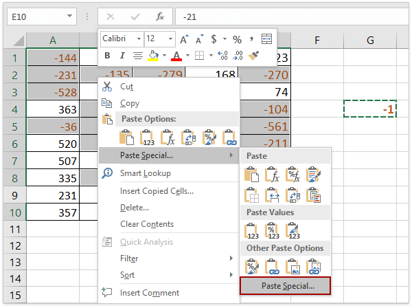
(1) Držení Ctrl klíč, můžete vybrat všechna záporná čísla kliknutím na ně jeden po druhém;
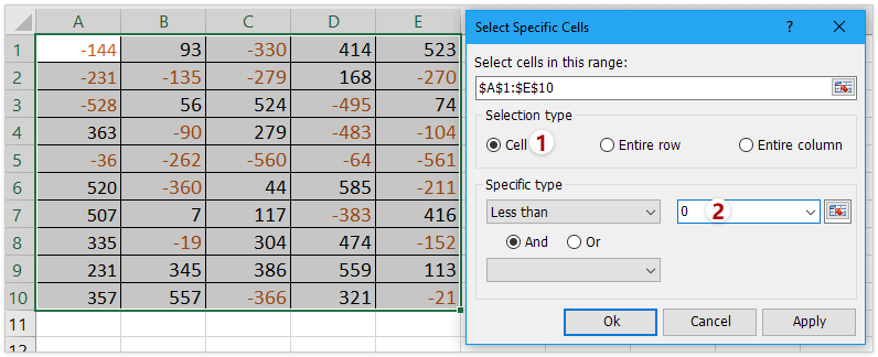
(2) Pokud máte nainstalovaný program Kutools pro Excel, můžete jej použít Vyberte speciální buňky funkce pro rychlý výběr všech záporných čísel. Vyzkoušejte zdarma!
3. A a Vložte speciální Zobrazí se dialogové okno, vyberte Zobrazit vše možnost od Pastavyberte Násobit možnost od Operace, Klepněte na tlačítko OK. Viz snímek obrazovky:

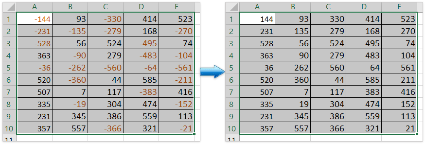
4. Všechna vybraná záporná čísla budou převedena na kladná čísla. Odstraňte číslo -1, jak potřebujete. Viz snímek obrazovky:

Snadno změňte záporná čísla na kladná ve specifikovaném rozsahu v aplikaci Excel
Ve srovnání s ručním odstraněním negativního znaménka z buněk, Kutools pro Excel Změnit znaménko hodnot Tato funkce poskytuje extrémně snadný způsob, jak rychle změnit všechna záporná čísla na pozitivní při výběru. Získejte 30denní plnohodnotnou bezplatnou zkušební verzi!
Kutools pro Excel - Supercharge Excel s více než 300 základními nástroji. Užijte si plnohodnotnou 30denní zkušební verzi ZDARMA bez nutnosti kreditní karty! Get It Now
Rychle a snadno změňte záporná čísla na pozitivní pomocí Kutools pro Excel
Většina uživatelů aplikace Excel nechce používat kód VBA, existují nějaké rychlé triky pro změnu záporných čísel na pozitivní? Kutools pro Excel vám pomůže snadno a pohodlně toho dosáhnout.
Kutools pro Excel - Supercharge Excel s více než 300 základními nástroji. Užijte si plnohodnotnou 30denní zkušební verzi ZDARMA bez nutnosti kreditní karty! Get It Now
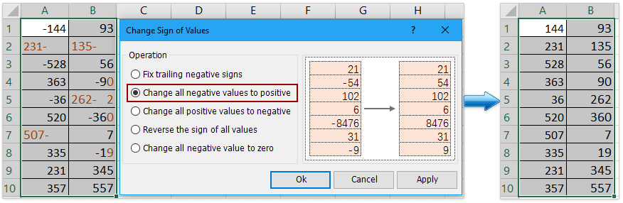
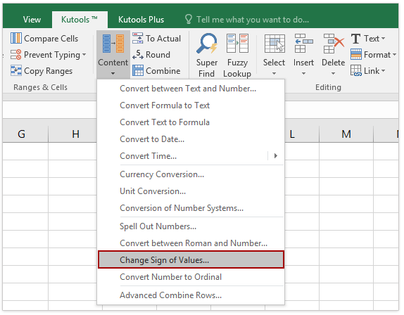
1. Vyberte rozsah včetně záporných čísel, která chcete změnit, a klikněte Kutools > Obsah > Změnit znaménko hodnot.
2. Check Změňte všechny záporné hodnoty na kladné pod Operace, a klepněte na tlačítko Ok. Viz snímek obrazovky:
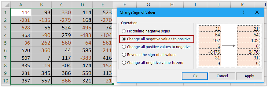
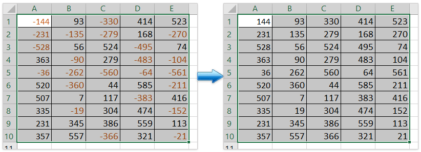
Nyní uvidíte, jak se všechna záporná čísla změní na kladná čísla, jak je uvedeno níže:
Poznámka: S tím Změnit znaménko hodnot Pomocí funkce můžete také opravit koncové záporné znaménka, změnit všechna kladná čísla na záporná, obrátit znaménko všech hodnot a změnit všechny záporné hodnoty na nulu. Vyzkoušejte zdarma!
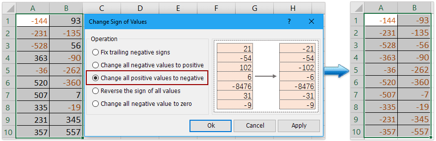
(1) Rychle změňte všechny kladné hodnoty na záporné ve stanoveném rozsahu:
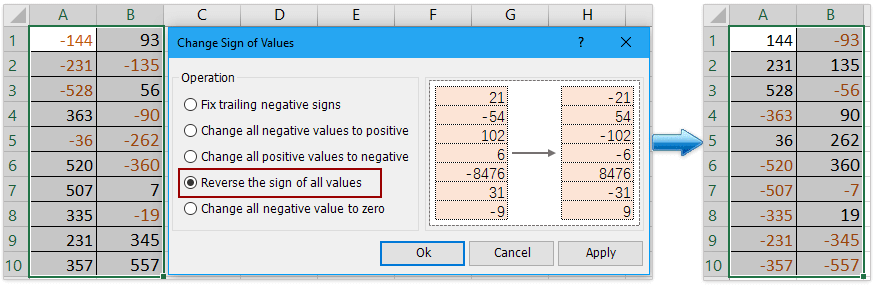
(2) Snadno obraťte znaménko všech hodnot ve specifikovaném rozsahu:
(3) Snadno změňte všechny záporné hodnoty na nulu ve specifikovaném rozsahu:

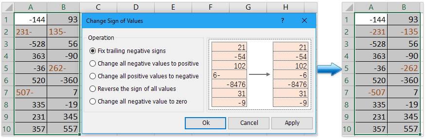
(4) Snadno opravte koncové negativní znaménka ve specifikovaném rozsahu:
Pomocí kódu VBA převedete všechna záporná čísla rozsahu na kladná
Jako profesionál v Excelu můžete také spustit kód VBA a změnit záporná čísla na kladná čísla.
1. Stisknutím kláves Alt + F11 otevřete okno Microsoft Visual Basic pro aplikace.
2. Zobrazí se nové okno. Klepněte na Vložit > Modul, poté vložte do modulu následující kódy:
Sub Positive
Dim Cel As Range
For Each Cel In Selection
If IsNumeric(Cel.Value) Then
Cel.Value = Abs(Cel.Value)
End If
Next Cel
End Sub3. Pak klikněte na tlačítko Běh nebo stiskněte tlačítko F5 klíč ke spuštění aplikace a všechna záporná čísla budou změněna na kladná čísla. Viz snímek obrazovky:
Ukázka: Změňte záporná čísla na kladná nebo naopak pomocí Kutools pro Excel
Související články
Reverzní znaky hodnot v buňkách
Když použijeme Excel, jsou v listu kladná i záporná čísla. Předpokládejme, že musíme změnit kladná čísla na záporná a naopak. Samozřejmě je můžeme změnit ručně, ale pokud je třeba změnit stovky čísel, tato metoda není dobrá volba. Existují nějaké rychlé triky, jak tento problém vyřešit?
Změňte kladná čísla na záporná
Jak můžete rychle změnit všechna kladná čísla nebo hodnoty na negativní v aplikaci Excel? Následující metody vám pomohou rychle změnit všechna kladná čísla na záporná v aplikaci Excel.
Opravte koncové negativní znaky v buňkách
Z některých důvodů možná budete muset opravit koncové negativní znaky v buňkách v aplikaci Excel. Například číslo s koncovými zápornými znaménky by bylo jako 90-. Jak v této podmínce můžete rychle opravit koncové negativní znaménka odstraněním koncové negativní značky zprava doleva? Zde je několik rychlých triků, které vám mohou pomoci.
Změňte záporné číslo na nulu
Povedu vás, abyste ve výběru změnili všechna záporná čísla na nuly najednou.
Nejlepší kancelářské nástroje produktivity
Kutools pro Excel - pomůže vám vyniknout před davem
Kutools pro Excel se může pochlubit více než 300 funkcemi, Zajištění toho, že to, co potřebujete, je jen jedno kliknutí...
")
Záložka Office - Povolte čtení a úpravy na záložkách v Microsoft Office (včetně Excelu)
- Jednu sekundu přepnete mezi desítkami otevřených dokumentů!
- Snižte stovky kliknutí myší každý den, sbohem s myší rukou.
- Zvyšuje vaši produktivitu o 50% při prohlížení a úpravách více dokumentů.
- Přináší efektivní karty do Office (včetně Excelu), stejně jako Chrome, Edge a Firefox.
")