Přejít k hlavnímu obsahu

Jak vypsat všechny možné kombinace z jednoho sloupce v Excelu?

Autor: Xiaoyang Naposledy změněno: 2023-04-10

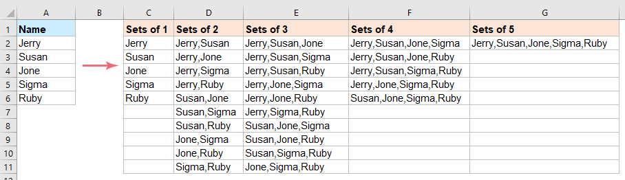
Pokud chcete vrátit všechny možné kombinace z dat jednoho sloupce, abyste získali výsledek, jak je zobrazen níže na snímku obrazovky, máte nějaké rychlé způsoby, jak se s tímto úkolem v Excelu vypořádat?

Vypište všechny možné kombinace z jednoho sloupce se vzorci

Seznam všech možných kombinací z jednoho sloupce s kódem VBA


Vypište všechny možné kombinace z jednoho sloupce se vzorci

Následující maticové vzorce vám mohou pomoci dosáhnout tohoto úkolu, proveďte prosím krok za krokem:

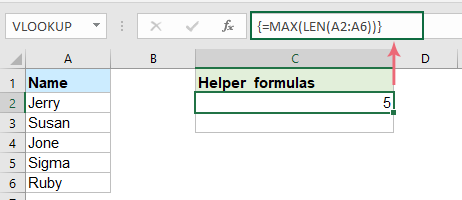
1. Nejprve byste měli vytvořit dvě buňky pomocného vzorce. Do buňky C1 zadejte níže uvedený vzorec a stiskněte Ctrl + Shift + Enter klíče k získání výsledku:

=MAX(LEN(A2:A6))
Poznámka: V tomto vzorci A2: A6 je seznam buněk, u kterých chcete vypsat jejich kombinace.

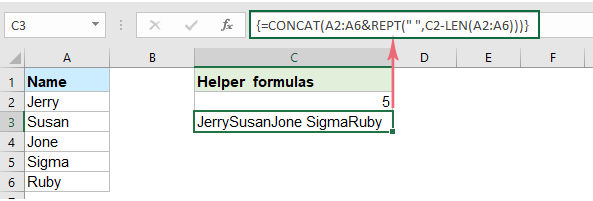
2. Do buňky C2 zadejte následující vzorec a stiskněte Ctrl + Shift + Enter kláves dohromady, abyste získali druhý výsledek, viz snímek obrazovky:

=CONCAT(A2:A6&REPT(" ",C2-LEN(A2:A6)))
Poznámka: V tomto vzorci A2: A6 je seznam buněk, u kterých chcete vypsat jejich kombinace, C2 je buňka obsahuje vzorec, který jste vytvořili v kroku 1.

3. Poté zkopírujte a vložte následující vzorec do buňky D2 a stiskněte Ctrl + Shift + Enter společně získáte první výsledek, viz screenshot:

=IF(ROW()>2^(COUNTA(A$2:A$6)),"",TEXTJOIN(" + ",TRUE,IF(MID(TEXT(DEC2BIN(ROW()-1),REPT("0",COUNTA($A$2:$A$6))),ROW(INDIRECT("1:"&COUNTA($A$2:$A$6))),1)+0,TRIM(MID($C$3,(ROW(INDIRECT("1:"&COUNTA($A$2:$A$6)))-1)*$C$2+1,$C$2)),"")))
Poznámka: V tomto vzorci A2: A6 je seznam buněk, u kterých chcete vypsat jejich kombinace, C2 je buňka obsahuje vzorec, který jste vytvořili v kroku 1, C3 je buňka se vzorcem, který jste vytvořili v kroku 2, the + znak je oddělovač pro oddělení kombinací, můžete je změnit podle potřeby.

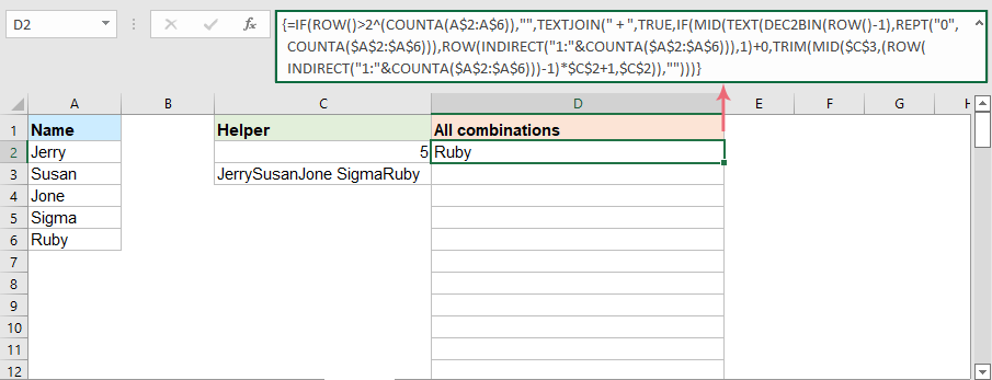
4. A pak vyberte tuto buňku vzorce a přetáhněte úchyt výplně dolů, dokud se neobjeví prázdné buňky. Nyní můžete vidět, že všechny kombinace dat zadaných sloupců jsou zobrazeny, jak je ukázáno níže:

Poznámka: Tento vzorec je k dispozici pouze v Office 2019, 365 a novějších verzích.

Seznam všech možných kombinací z jednoho sloupce s kódem VBA

Výše uvedené vzorce jsou k dispozici pouze pro novější verze aplikace Excel, pokud máte dřívější verze aplikace Excel, může vám pomoci následující kód VBA.

1. lis Alt + F11 současně otevřete Microsoft Visual Basic pro aplikace okno.

2. Potom klepněte na tlačítko Vložit > Modul, zkopírujte a vložte níže uvedený kód VBA do okna.

Kód VBA: Seznam všech možných kombinací z jednoho sloupce

Sub ConnectArr()
'Updateby ExtendOffice
Dim xDValue As Variant
Dim xOutRg As Range
Dim xDictionary As Object
Dim xF As Long
Dim xChar As String
xDValue = Range("A2:A6").Value 'the data range
Set xOutRg = Range("C1") 'output range
xChar = "," 'separator
For xF = 1 To UBound(xDValue)
    Set xDictionary = CreateObject("Scripting.Dictionary")
    xDictionary(0) = "Sets of " & xF
    Call ConnectValue(xDValue, xDictionary, 0, xF, 0, "", xChar)
    xOutRg.Offset(0, xF - 1).Resize(xDictionary.Count).Value = WorksheetFunction.Transpose(xDictionary.Items)
    Set xDictionary = Nothing
Next
End Sub
Sub ConnectValue(ByRef pDValue, ByRef pDictionary, ByRef pLevel, ByVal pMaxLevel, ByVal pIndex, ByVal pValue, ByVal pChar)
Dim xF As Long
If pLevel = pMaxLevel Then
    pDictionary(pDictionary.Count + 1) = pValue
    Exit Sub
End If
For xF = pIndex + 1 To UBound(pDValue)
    If pValue = "" Then
        Call ConnectValue(pDValue, pDictionary, pLevel + 1, pMaxLevel, xF, pDValue(xF, 1), pChar)
    Else
        Call ConnectValue(pDValue, pDictionary, pLevel + 1, pMaxLevel, xF, pValue & pChar & pDValue(xF, 1), pChar)
    End If
Next
End Sub
Poznámka: Ve výše uvedeném kódu:
  • A2: A6: je seznam dat, která chcete použít;
  • C1: je výstupní buňka;
  • ,: oddělovač pro oddělení kombinací.

3. A pak stiskněte F5 klíč k provedení tohoto kódu. Všechny kombinace z jednoho sloupce jsou uvedeny jako níže uvedený snímek obrazovky:

Nejlepší nástroje pro produktivitu v kanceláři

🤖 Kutools AI asistent: Revoluční analýza dat založená na: Inteligentní provedení   |  Generovat kód  |  Vytvořte vlastní vzorce  |  Analyzujte data a generujte grafy  |  Vyvolejte funkce Kutools...
Populární funkce: Najít, zvýraznit nebo identifikovat duplikáty   |  Odstranit prázdné řádky   |  Kombinujte sloupce nebo buňky bez ztráty dat   |   Kolo bez vzorce ...
Super vyhledávání: Více kritérií VLookup    VLookup s více hodnotami  |   VLookup na více listech   |   Fuzzy vyhledávání ....
Pokročilý rozevírací seznam: Rychle vytvořte rozevírací seznam   |  Závislý rozbalovací seznam   |  Vícenásobný výběr rozevíracího seznamu ....
Správce sloupců: Přidejte konkrétní počet sloupců  |  Přesunout sloupce  |  Přepnout stav viditelnosti skrytých sloupců  |  Porovnejte rozsahy a sloupce ...
Doporučené funkce: Zaměření mřížky   |  Návrhové zobrazení   |   Velký Formula Bar    Správce sešitů a listů   |  Knihovna zdrojů (Automatický text)   |  Výběr data   |  Zkombinujte pracovní listy   |  Šifrovat/dešifrovat buňky    Odesílat e-maily podle seznamu   |  Super filtr   |   Speciální filtr (filtr tučné/kurzíva/přeškrtnuté...) ...
Top 15 sad nástrojů12 Text Tools (doplnit text, Odebrat znaky, ...)   |   50+ Graf Typ nemovitosti (Ganttův diagram, ...)   |   40+ Praktické Vzorce (Vypočítejte věk na základě narozenin, ...)   |   19 Vložení Tools (Vložte QR kód, Vložit obrázek z cesty, ...)   |   12 Konverze Tools (Čísla na slova, Přepočet měny, ...)   |   7 Sloučit a rozdělit Tools (Pokročilé kombinování řádků, Rozdělit buňky, ...)   |   ... a více

Rozšiřte své dovednosti Excel pomocí Kutools pro Excel a zažijte efektivitu jako nikdy předtím. Kutools for Excel nabízí více než 300 pokročilých funkcí pro zvýšení produktivity a úsporu času.  Kliknutím sem získáte funkci, kterou nejvíce potřebujete...

Popis


Office Tab přináší do Office rozhraní s kartami a usnadňuje vám práci

  • Povolte úpravy a čtení na kartách ve Wordu, Excelu, PowerPointu, Publisher, Access, Visio a Project.
  • Otevřete a vytvořte více dokumentů na nových kartách ve stejném okně, nikoli v nových oknech.
  • Zvyšuje vaši produktivitu o 50%a snižuje stovky kliknutí myší každý den!
Comments (11)
No ratings yet. Be the first to rate!
This comment was minimized by the moderator on the site
Hi Skyyang,

Not sure if you are still active on this thread. But just taking a chance in case. I am not very familiar with VBA coding and am stuck in a situation where I need code to tackle one situation in my project. I need to create a unique combination from the list of variables mentioned in "SHEET1" cells "A2:A20". The combination will be of 2 variables listed in the row starting from A2 in SHEET2. And a list with 3 variable combinations listed in the row starting from A2 in SHEET3.

Thanks in advance.
This comment was minimized by the moderator on the site
Hello,
Nice job!
But I'm interested to find just the "Sets of 2", as in your example, e.g. a list of players who have to play matches with each other :).
Thank you.
This comment was minimized by the moderator on the site
Hello, Iulian,
To solve your problem, please apply the below code:
Note: your names should be start at A2 cell, and the result will be placed at C2 cell.
Sub name_by_name()
    Dim i As Long, j As Long, lr As Long
    With ActiveSheet
        lr = .Cells(Rows.Count, 1).End(xlUp).Row
        For i = 2 To lr
            For j = i + 1 To lr
                .Cells(Rows.Count, 3).End(xlUp).Offset(1, 0) = _
                  .Cells(i, 1).Value & ", " & .Cells(j, 1).Value
            Next j
        Next i
    End With
End Sub


Please have a try, hope it can help you!

https://www.extendoffice.com/images/stories/comments/comment-skyyang/2023-comment/combinations-1.png
This comment was minimized by the moderator on the site
Hello, I have a list of 30 items in a column and the code doesn't seem to be able to handle that, what is the max number of items allowed for the code to work? is there a way to make a long list work?
This comment was minimized by the moderator on the site
Hello, Lynn,
Yes, as you said, if the number of cells are greater than 20, the code will not work well.
Sorry for that inconvenience.

With this code, it will pop out an alert if the number of cells is greater than 20.
Sub ConnectArr()
'Updateby ExtendOffice
Dim xDValue As Variant
Dim xOutRg As Range
Dim xDictionary As Object
Dim xF As Long
Dim xChar As String
Dim xAddress As String
xAddress = "A1:A20" 'the data range
If Range(xAddress).Count > 20 Then
    MsgBox "The number of cells can't greater than 20!"
    Exit Sub
End If
xDValue = Range(xAddress).Value
Set xOutRg = Range("C1") 'output range
xChar = "," 'separator
For xF = 1 To UBound(xDValue)
    Set xDictionary = CreateObject("Scripting.Dictionary")
    xDictionary(0) = "Sets of " & xF
    Call ConnectValue(xDValue, xDictionary, 0, xF, 0, "", xChar)
    xOutRg.Offset(0, xF - 1).Resize(xDictionary.Count).Value = WorksheetFunction.Transpose(xDictionary.Items)
    Set xDictionary = Nothing
Next
End Sub
Sub ConnectValue(ByRef pDValue, ByRef pDictionary, ByRef pLevel, ByVal pMaxLevel, ByVal pIndex, ByVal pValue, ByVal pChar)
Dim xF As Long
If pLevel = pMaxLevel Then
    pDictionary(pDictionary.Count + 1) = pValue
    Exit Sub
End If
For xF = pIndex + 1 To UBound(pDValue)
    If pValue = "" Then
        Call ConnectValue(pDValue, pDictionary, pLevel + 1, pMaxLevel, xF, pDValue(xF, 1), pChar)
    Else
        Call ConnectValue(pDValue, pDictionary, pLevel + 1, pMaxLevel, xF, pValue & pChar & pDValue(xF, 1), pChar)
    End If
Next
End Sub

This comment was minimized by the moderator on the site
I really like the method but values bottom out at the 511th row and you get #NUM! if you have more than 6 entries in column A. I'm wondering if someone might consider helping me to adjust the formula so that the resulting values calculate beyond the 511th row? Thank you very much! =)
This comment was minimized by the moderator on the site
Hello,
Yes, as you said, the formula will stop work in row 511. So, here, you can appy the VBA code in this article.
Or if you want to list all possible combinations into single one column, please apply the below code:
Note: In the code, A2 is the first cell contains the data you want to use, you should change the cell reference A2 and A to your own. After running the code, all combinations will be listed in the next column of the data list.
Sub allcombination()
Dim Ray As Variant, n As Long, nn As Long, Allnum As String, c As Long
Dim Res As Long, obit, oSt, ipc, Tot As Long, oPst As Long, sNum As String
Ray = Application.Transpose(Range(Range("A2"), Range("A" & Rows.Count).End(xlUp)))
sNum = Join(Evaluate("TRANSPOSE(ROW(" & 1 & ":" & UBound(Ray) & "))"), ",")
For n = 1 To UBound(Ray)
    Tot = Tot + Application.Combin(UBound(Ray), n)
Next n
ReDim Oval(1 To Tot)
ReDim nRay(1 To Tot - UBound(Ray))
Do Until Allnum = sNum
   If c < UBound(Ray) Then
       For n = 1 To UBound(Ray)
             c = c + 1: Oval(c) = n
       Next n
   Else
       For n = 1 To UBound(Ray)
             Res = Res + 1
             obit = Oval(Res)
             oSt = Split(obit, ",")(UBound(Split(obit, ",")))
                For nn = oSt + 1 To UBound(Ray)
                    c = c + 1
                    Allnum = obit & "," & nn
                    Oval(c) = Allnum
                Next nn
         Next n
   End If
Loop
Dim s As Variant, nStr As String
    For oPst = UBound(Ray) + 1 To UBound(Oval)
        For Each s In Split(Oval(oPst), ",")
            nStr = nStr & IIf(nStr = "", Ray(s), "," & Ray(s))
        Next s
            nRay(oPst - UBound(Ray)) = nStr: nStr = ""
  Next oPst
Range("B1").Resize(UBound(nRay)).Value = Application.Transpose(nRay)
End Sub

Please have a try, hope it can help you! 🙂
This comment was minimized by the moderator on the site
Dear skyyang:

Thank you very much for your help and the code. It's invaluable and I'm grateful.

I'm relatively new to VB scripting, consequently not very adept at coding the language.

Just a point or two:

- Your suggested code doesn't generate single entries (e.g. Ruby, or...)
- The original ordering as highlighted in the animated graphic in Step 4 disappeared.

I will go through your code to try my hand at calibrating it so that the above points are outputted, but I was wondering if you had any quick advice or suggestion(s) that could address them.

Thank you again for your kind help. I really appreciate it. =)

My best.
This comment was minimized by the moderator on the site
Dear skyyang:

First, thank you very much for your code solution. I am grateful! =)

I wrote a reply yesterday but the system seems not to have posted it for unknown reasons. I hope this one gets through.

Your code generates output that I am interested in. I had just a couple of observations and then a question:

1) The code doesn't generate the individual entries alone.
2) The original ordering seen in the animated graphic in Step 4 is lost.

From your code is there a way to also include the single entries and to mirror the original ordering format from Step 4. I'm rather new to VB scripting.

Again, thank you so much for your invaluable help. I really appreciate it.

My best.
This comment was minimized by the moderator on the site
Dear skyyang:

This is wonderful. Thank you, this helps me out immensely. I am very grateful.

Just a couple observations I noticed after generating the VB code you provided was that the singletons (for lack of a better term), like just "Ruby", would get omitted, and the resulting (columnal) ordering no longer corresponded to the original ordering generated in Step 4 animated graphic.

Do you happen to have any quick suggestions about how I could tweak your code to also include the "singletons" and for matching the same ordering as in Step 4? I will try to wrangle the workaround but regrettably I'm fairly new to VB scripting.

Thanks again! I really appreciate it.

My best. =)
This comment was minimized by the moderator on the site
Hello, ffuuzz
In this case, you can try the vba code in our article, all possible combinations will be listed into separated columns, please try:
Sub ConnectArr()
'Updateby ExtendOffice
Dim xDValue As Variant
Dim xOutRg As Range
Dim xDictionary As Object
Dim xF As Long
Dim xChar As String
xDValue = Range("A2:A6").Value 'the data range
Set xOutRg = Range("C1") 'output range
xChar = "," 'separator
For xF = 1 To UBound(xDValue)
    Set xDictionary = CreateObject("Scripting.Dictionary")
    xDictionary(0) = "Sets of " & xF
    Call ConnectValue(xDValue, xDictionary, 0, xF, 0, "", xChar)
    xOutRg.Offset(0, xF - 1).Resize(xDictionary.Count).Value = WorksheetFunction.Transpose(xDictionary.Items)
    Set xDictionary = Nothing
Next
End Sub
Sub ConnectValue(ByRef pDValue, ByRef pDictionary, ByRef pLevel, ByVal pMaxLevel, ByVal pIndex, ByVal pValue, ByVal pChar)
Dim xF As Long
If pLevel = pMaxLevel Then
    pDictionary(pDictionary.Count + 1) = pValue
    Exit Sub
End If
For xF = pIndex + 1 To UBound(pDValue)
    If pValue = "" Then
        Call ConnectValue(pDValue, pDictionary, pLevel + 1, pMaxLevel, xF, pDValue(xF, 1), pChar)
    Else
        Call ConnectValue(pDValue, pDictionary, pLevel + 1, pMaxLevel, xF, pValue & pChar & pDValue(xF, 1), pChar)
    End If
Next
End Sub
There are no comments posted here yet
Please leave your comments in English
Posting as Guest
×
Rate this post:
0   Characters
Suggested Locations