Přejít k hlavnímu obsahu

Jak najít n-tou prázdnou buňku v aplikaci Excel?

Jak můžete najít a vrátit hodnotu n-té prázdné buňky ze sloupce nebo řádku v aplikaci Excel? V tomto článku budu hovořit o některých užitečných vzorcích pro vyřešení tohoto úkolu.

Najděte a vraťte n-tou neprázdnou hodnotu buňky ze sloupce se vzorcem

Najděte a vraťte n-tou neprázdnou hodnotu buňky z řádku pomocí vzorce


šipka modrá pravá bublina Najděte a vraťte n-tou neprázdnou hodnotu buňky ze sloupce se vzorcem

Například mám sloupec dat, jak ukazuje následující snímek obrazovky, nyní z tohoto seznamu dostanu třetí hodnotu prázdné buňky.

doc najít n-té neprázdné 1

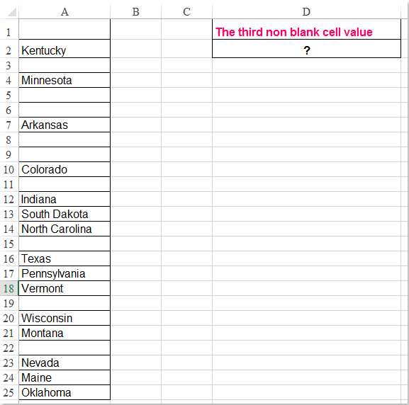
Zadejte prosím tento vzorec: =INDEX($A$1:$A$25,SMALL(ROW($A$1:$A$25)+(100*($A$1:$A$25="")), 3))&"" do prázdné buňky, kam chcete odeslat výsledek, například D2, a poté stiskněte Ctrl + Shift + Enter společně získáte správný výsledek, viz screenshot:

doc najít n-té neprázdné 2

Poznámka: Ve výše uvedeném vzorci, A1: A25 je seznam dat, který chcete použít, a číslo 3 označuje třetí hodnotu neprázdné buňky, kterou chcete vrátit, pokud chcete získat druhou neprázdnou buňku, stačí změnit číslo 3 na 2 podle potřeby.


šipka modrá pravá bublina Najděte a vraťte n-tou neprázdnou hodnotu buňky z řádku pomocí vzorce

Pokud chcete najít a vrátit n-tou prázdnou hodnotu buňky v řádku, může vám pomoci následující vzorec, postupujte takto:

Zadejte tento vzorec: =INDEX($A$1:$M$1,SMALL(IF($A$1:$M$1<>"",COLUMN($A$1:$M$1)-COLUMN($A$1)+1),4)) do prázdné buňky, kde chcete vyhledat výsledek, a stiskněte Ctrl + Shift + Enter společně získáte výsledek, viz screenshot:

doc najít n-té neprázdné 3

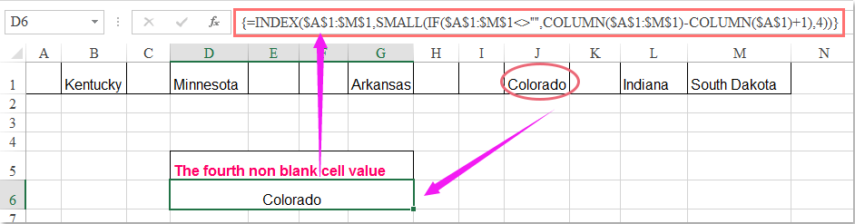
Poznámka: Ve výše uvedeném vzorci A1: M1 je hodnota řádku, který chcete použít, a číslo 4 je čtvrtá hodnota prázdné buňky, kterou chcete vrátit, pokud chcete získat druhou neprázdnou buňku, stačí změnit číslo 4 na 2 podle potřeby.

Nejlepší nástroje pro produktivitu v kanceláři

🤖 Kutools AI asistent: Revoluční analýza dat založená na: Inteligentní provedení   |  Generovat kód  |  Vytvořte vlastní vzorce  |  Analyzujte data a generujte grafy  |  Vyvolejte funkce Kutools...
Populární funkce: Najít, zvýraznit nebo identifikovat duplikáty   |  Odstranit prázdné řádky   |  Kombinujte sloupce nebo buňky bez ztráty dat   |   Kolo bez vzorce ...
Super vyhledávání: Více kritérií VLookup    VLookup s více hodnotami  |   VLookup na více listech   |   Fuzzy vyhledávání ....
Pokročilý rozevírací seznam: Rychle vytvořte rozevírací seznam   |  Závislý rozbalovací seznam   |  Vícenásobný výběr rozevíracího seznamu ....
Správce sloupců: Přidejte konkrétní počet sloupců  |  Přesunout sloupce  |  Přepnout stav viditelnosti skrytých sloupců  |  Porovnejte rozsahy a sloupce ...
Doporučené funkce: Zaměření mřížky   |  Návrhové zobrazení   |   Velký Formula Bar    Správce sešitů a listů   |  Knihovna zdrojů (Automatický text)   |  Výběr data   |  Zkombinujte pracovní listy   |  Šifrovat/dešifrovat buňky    Odesílat e-maily podle seznamu   |  Super filtr   |   Speciální filtr (filtr tučné/kurzíva/přeškrtnuté...) ...
Top 15 sad nástrojů12 Text Tools (doplnit text, Odebrat znaky, ...)   |   50+ Graf Typ nemovitosti (Ganttův diagram, ...)   |   40+ Praktické Vzorce (Vypočítejte věk na základě narozenin, ...)   |   19 Vložení Tools (Vložte QR kód, Vložit obrázek z cesty, ...)   |   12 Konverze Tools (Čísla na slova, Přepočet měny, ...)   |   7 Sloučit a rozdělit Tools (Pokročilé kombinování řádků, Rozdělit buňky, ...)   |   ... a více

Rozšiřte své dovednosti Excel pomocí Kutools pro Excel a zažijte efektivitu jako nikdy předtím. Kutools for Excel nabízí více než 300 pokročilých funkcí pro zvýšení produktivity a úsporu času.  Kliknutím sem získáte funkci, kterou nejvíce potřebujete...

Popis


Office Tab přináší do Office rozhraní s kartami a usnadňuje vám práci

  • Povolte úpravy a čtení na kartách ve Wordu, Excelu, PowerPointu, Publisher, Access, Visio a Project.
  • Otevřete a vytvořte více dokumentů na nových kartách ve stejném okně, nikoli v nových oknech.
  • Zvyšuje vaši produktivitu o 50%a snižuje stovky kliknutí myší každý den!
Comments (10)
No ratings yet. Be the first to rate!
This comment was minimized by the moderator on the site
CIAO STO CERCANDO DI APPLICARE LA TUA FORMULA MA NON MI FUNZIONA, DOVE STO SBAGLIANDO?
=INDICE($K$37:$K$88;MIN(RIGHE($K$37:$K$88)+RIGHE(100*($K$37:$K$88=""));6))&""
DEVO VISUALIZZARE L'ENNESIMA RIGA DIVERSA DA VUOTO

GRAzie
This comment was minimized by the moderator on the site
=INDICE($K$37:$K$88;MIN(RIGHE($K$37:$K$88)+(100*($K$37:$K$88=""));6))&""
This comment was minimized by the moderator on the site
I'm running this formula on a ~400 row sheet with around 20 blanks mixed throughout the data, and it's working perfectly EXCEPT when I fill the series down, it sometimes duplicates a row for some reason. For example, it seems to think a value is somehow simultaneously the 331st non-blank and the 332nd.

Things I've noticed:
-Duplications always happen in pairs (ex. 331 and 332 are duplicates, 333 and 334 will also be), then it goes back to normal for a while.
-Raw data also has blanks in pairs, but not corresponding to the duplicates
-No duplications occur in the first 94 rows, but they happen every 33-35 rows after that
-Does not appear to be linked to the value in the cell being duplicated
-I have entered as an array and as a standard formula, no difference in function

For reference, here's my actual formula:

=INDEX('PO Raw Data'!CR:CR,SMALL(ROW('PO Raw Data'!CR:CR)+(100*('PO Raw Data'!CR:CR="")),$W2)&"")

Note $W2 refers to a helper column and counts up as the data set is filled down, but only because I couldn't get it to count up when I just used a number instead of cell reference.
When I've replaced that cell reference (ex. $W2) with the appropriate number, same result.


Any thoughts on what I can do to fix that?
This comment was minimized by the moderator on the site
very helpful,
although when I return the nth non blank cell in a column set to DATE, the returned value appears as number(general number).formatting the cell into DATE also doesn't change the result. could you please give me a hand!
thanks a lot
This comment was minimized by the moderator on the site
Hello, Shirazi,
Sorry, maybe there is no direct formula for you to get the date format.

If someone else has the solution, please comment here.
This comment was minimized by the moderator on the site
Hi everyone!


Could you also help me return the row number of the second, third non-blank cell?


Please help me.
This comment was minimized by the moderator on the site
Hello, John,
the following formula can help you to get all the row numbers of the non-blank cells, please try it, thank you!
=IFERROR(ROW(INDEX($A$1:$A$12,SMALL(INDEX(NOT(ISBLANK($A$1:$A$12))*ROW($A$1:$A$12),0),COUNTBLANK($A$1:$A$12)+ROW(A1)))),"")
This comment was minimized by the moderator on the site
Hey everyone,

I have a table with numerous columns and rows. The rows have range names, and a description/location at the beginning of the row range with its own range, example "Building No.s". There are multiple Row Ranges/ Buildings. There are headers at the top of each columns for specific "Building Assembly Types". The table content is numeric quantities for each type "Building Assembly Type" for each specific "Building" description/location. There could be as many as (100) "Building Assembly Types" column headers but I will limit the assemblies to (10) per row range, so there will be numerous blank cells in each "Building No." range.

I have other summary tables set up for each "Building" that I want to pull the non-blank cells quantities to, along with the corresponding header "Assembly Type" for each "Building" with a (10) max "Assemblies" per page.

I can identify the non-blank cell quantities by use of the array formula above for rows. The problem I am having is identifying the header that corresponds to it.

Ultimately if I can identify the "Assembly" header, I can always index the "Quantities" once I have the header "Assembly" identified for each "Building". Then I would be able do a lookup for all the parts associated with each "Assembly" type for that "Building" from my Assembly parts database and multiply it times the "Quantity" of each assembly type.

Hopefully this makes since and someone can help.
This comment was minimized by the moderator on the site
Hello, I am looking for the third blank row in a column and I copied your formula and just changed the range from $A$1:$A:$25 to my range $D$306:$D$354. But when I change the range I get #REF! as my answer. I already converted to an array, control-shift-enter. Now the cell range I am referencing has formulas in them, so could that be why I am getting #REF. Your formula: =INDEX($A$1:$A$25,SMALL(ROW($A$1:$A$25)+(100*($A$1:$A$25="")), 3))&"" My formula: =INDEX($D$306:$D$354,SMALL(ROW($D$306:$D$354)+(1*($D$306:$D$354="")), 2))&"" Thanks, Noel
This comment was minimized by the moderator on the site
you have put the 1 instead of 100 therefore answered was wrong. please use below formula

INDEX($D$306:$D$354,SMALL(ROW($D$306:$D$354)+(100*($D$306:$D$354="")), 3))&"" than ctrl + shift+enter
There are no comments posted here yet
Please leave your comments in English
Posting as Guest
×
Rate this post:
0   Characters
Suggested Locations